library(skewt)
library(MASS)
library(copula)13 Simulations
Simulations are a very powerful technique widely used in risk forecasting. In financial analysis, simulations become useful when dealing with complex models that lack analytical solutions, such as pricing exotic options, calculating Value-at-Risk for non-linear portfolios, or stress testing under extreme market scenarios. They allow us to handle path-dependent instruments, model portfolio diversification effects, and capture the impact of tail events that traditional models might miss.
For example, we use simulations to evaluate the accuracy of various models, provide intuition on how models work, and provide analysis that otherwise would require complicated mathematics. In risk management, simulations enable us to generate thousands of potential market scenarios and assess how our portfolios might perform under each, providing insights that would be impossible to obtain through analytical methods alone. Advanced applications of simulations in risk management, including Value-at-Risk calculations and stress testing, are covered in Chapter 21.
When referring to simulations, we often use the term, Monte Carlo, after the statelet on the southern coast of France famous for casinos. We will use the terms simulation, Monte Carlo, and MC interchangeably.
When doing simulations, we ask a computer algorithm to replicate the real world. It is important to recognise the limitations of such an exercise.
To begin with, we are asking a computer to do something random, but computers are deterministic machines and cannot create something that is fully random. Instead, they produce something called a pseudorandom number, and they do that using an algorithm called a pseudorandom number generator. That is clumsy, and going forward, we will simply use the term random number generator or RNG.
Second, the world is much more complicated than any simulated representation of it. It is, therefore, important to recognise that a simulation is only a very crude approximation of what actually happens. Even if a simulation exercise appears to validate or reject something, that might not actually be true.
A random number generator creates a sequence of numbers, and when it has gone through the sequence, it starts again from the beginning. Therefore, if we know the random number \(x_i\) and know the random number generator, we also know the number \(x_{i+1}\) and indeed all the random numbers. In cryptography, if hackers can figure out an actual random number and knows the generator, they can maliciously decrypt all documents.
The number of different random numbers is known as the period. The default random number generator in R has a period of \(2^{19937}−1\), approximately \(10^{6001.64}\), which is more than enough for almost every possible application. And on the odd chance it is not sufficient, there are random number generators that can even create more.
The term seed refers to a particular starting point in the sequence of random numbers, and the command for setting the seed is set.seed(). Therefore, if one sets the seed to 1, one always gets the same random numbers. However, if one picks two instead, that is not simply the second number in the sequence.
13.1 Data and libraries
13.2 Random numbers
13.2.1 Basics
In Section 12.3, we discussed the various distributions built into R and the four forms of distribution: functions. The first letter of the function name indicates which of these four types, d for density, p for probability, q for quantile and r for random. The remainder of the name is the distribution, for example, for the normal and student-t:
To obtain one simulated standard normal, we call rnorm(n), where n is the number of different random numbers. For example:
rnorm(n = 1)[1] 0.99891rnorm(n = 5)[1] -0.8716787 -1.6605966 -0.4867118 -1.2460937 0.1212643Every time we call the function, we get a different random number:
rnorm(n = 1)[1] 0.3672856rnorm(n = 1)[1] -1.32923913.2.2 Seed
Generally, but not always, we want the random numbers to stay the same every time we run an algorithm. We are running some analysis, perhaps a risk calculation, and we want to get the same answer every time we run the program.
There are exceptions to this, and you may want the random numbers to change every time you call the algorithm. For example, if you use R to make a decision. Suppose you can not decide if you want to go to a movie. Then, you can run.
rnorm(1)[1] -0.9619334rnorm(1) < 0[1] TRUEifelse(rnorm(1) < 0, "stay at home", "go to a movie")[1] "go to a movie"ifelse(rnorm(1) < 0, "stay at home", "go to a movie")[1] "stay at home"ifelse(rnorm(1) < 0, "stay at home", "go to a movie")[1] "go to a movie"Since random number generators create a sequence of numbers that repeats, if we fix a place in the sequence, we always get the same random numbers. The way to do that is to set the seed in R set.seed()
rnorm(3)[1] 0.03012394 0.08541773 1.11661021rnorm(3)[1] -1.2188574 1.2673687 -0.7447816set.seed(666)
rnorm(3)[1] 0.7533110 2.0143547 -0.3551345set.seed(666)
rnorm(3)[1] 0.7533110 2.0143547 -0.3551345Having established how to control randomness through seeds, we can now explore the various probability distributions available in R for financial simulations.
13.3 Distributions
We will use several distributions, the normal (rnorm(n)), student-t (rt(n,df)), skewed student-t (rskt(n, df, gamma)), chi-square (rchisq(n,df)), the binomial (rbinom(n,size,prob)) and the Bernoulli, which is just rbinom(n, size = 1, prob = prob).
rnorm(n = 1)[1] 2.028168rt(n = 1, df = 3)[1] -1.968612rskt(n = 1, df = 3, gamma = 1)[1] -1.680305rchisq(n = 1, df = 2)[1] 0.05901815rbinom(n = 1, size = 1, prob = 0.5)[1] 0We can also plot some random numbers.
plot(rnorm(n = 100), pch = 16, col = 'blue')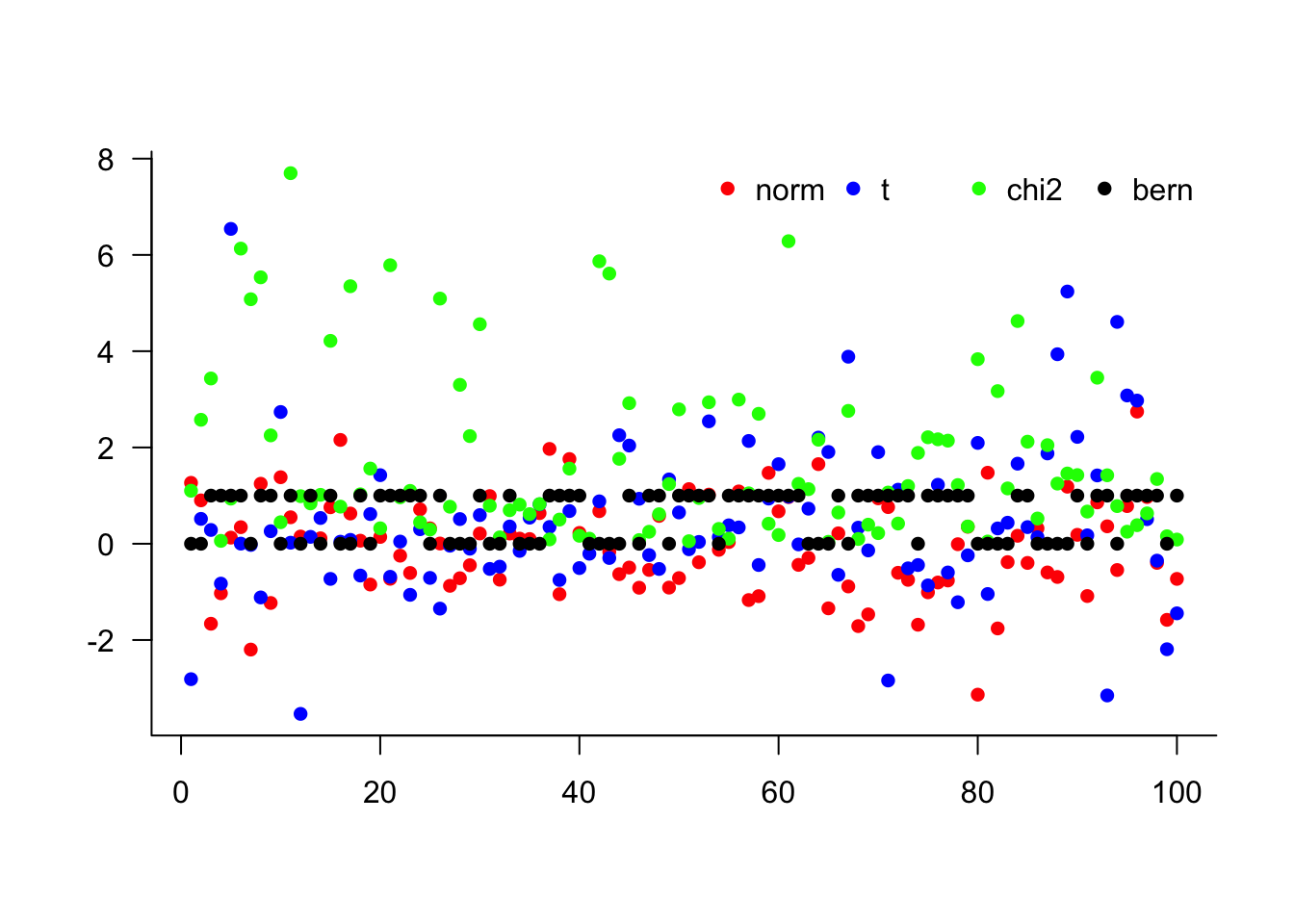
plot(rt(n = 100, df = 2), pch = 16, col = 'blue')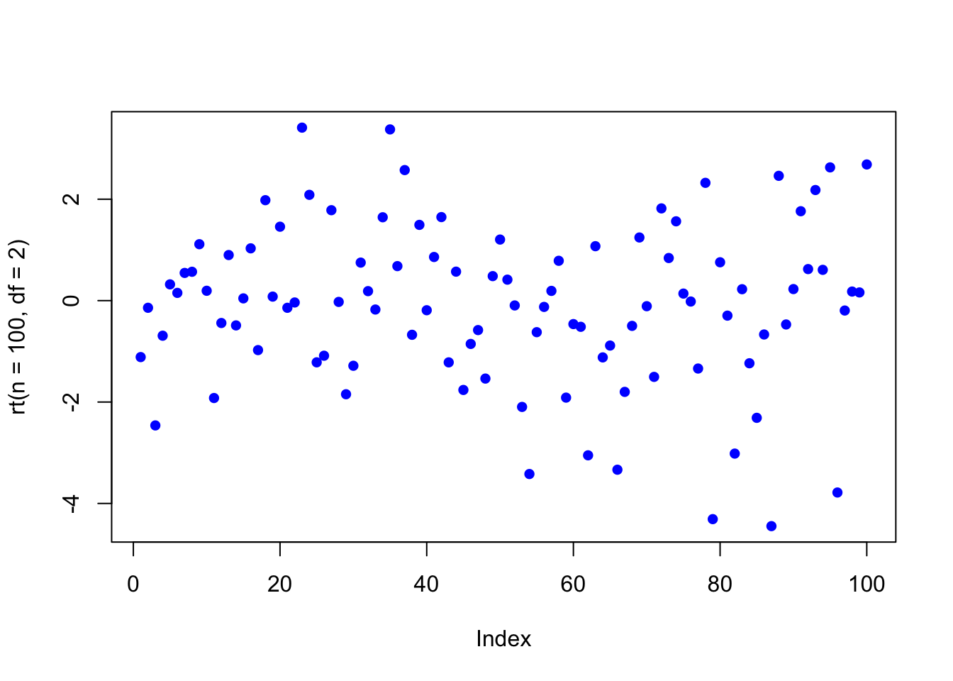
plot(rchisq(n = 100, df = 3), pch = 16, col = 'blue')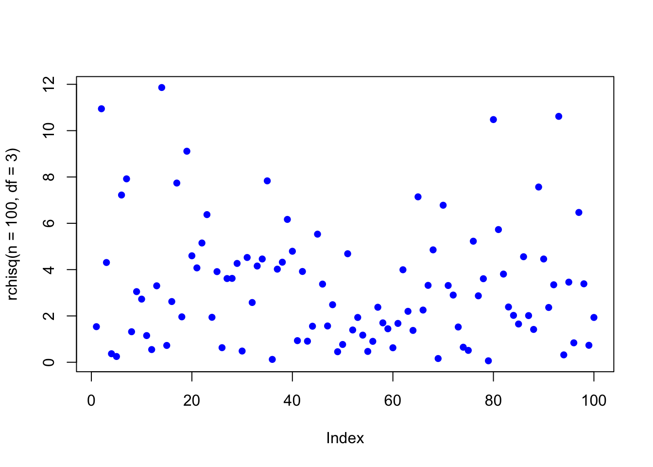
plot(rbinom(n = 100, size = 1, prob = 0.5), pch = 16, col = 'blue')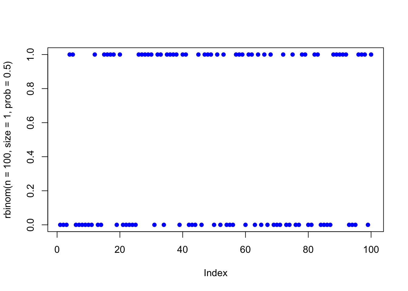
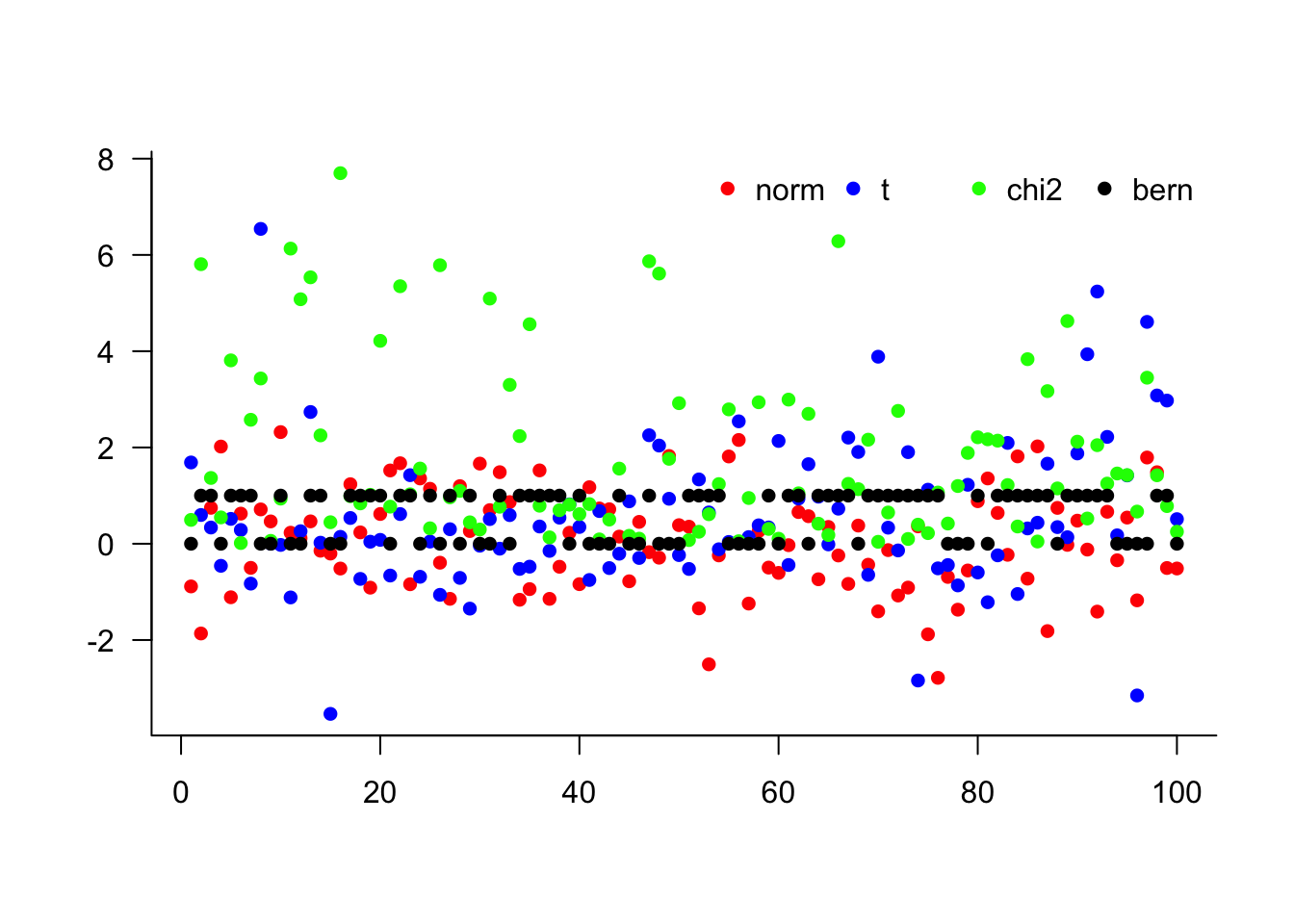
It might be better to see them all in the same plot.
x = cbind(
  rnorm(n = 100),
  rt(n = 100, df = 3),
  rchisq(n = 100, df = 2),
  rbinom(n = 100, size = 1, prob = 0.5)
)
head(x, 5)
[,1] [,2] [,3] [,4]
[1,] -0.8866582 1.6882590 0.4952933 0
[2,] -1.8641675 0.5972598 5.8075877 1
[3,] 0.7463817 0.3369926 1.3666579 1
[4,] 2.0189398 -0.4584508 0.5472326 0
[5,] -1.1117683 0.5166151 3.8093126 1matplot(x,
type = 'p',
pch = 16,
col = c("red", "blue", "green", "black"),
bty = 'l',
xlab = '',
ylab = '',
las = 1
)
legend("topright",
legend = c("norm", "t", "chi2", "bern"),
col = c("red", "blue", "green", "black"),
bty = 'n',
pch = 16,
horiz = TRUE
)
These examples demonstrate how to generate random numbers from different distributions. The next consideration is determining how many simulations are needed for reliable results.
13.4 Number of simulations
A key problem in simulations is to determine the number of necessary simulations. Pick too few, and one gets an inaccurate simulation estimate, and one wastes resources. The former problem is much more common. In a very special case, one over the square root of the number of simulations gives an estimate of the simulation accuracy, but that is only correct in a linear model. In that case, simulation is superfluous.
Below, we pick six simulation sizes, c(5,25,100,1e3,1e4,1e5), and see how well their mean and standard deviation compare to the known true value.
S = c(5, 25, 100, 1e3, 1e4, 1e5)
for(n in S){
  x = rnorm(n = n, mean = 1, sd = 2)
  if(n == S[1]){
    df = t(as.matrix(c(n, mean(x), sd(x))))
  }else{
    df = rbind(df, c(n, mean(x), sd(x)))
  }
}
df = as.data.frame(df)
names(df) = c("n", "mean", "sd")
df$meanError = df$mean - 1
df$sdError = df$sd - 2

print(df)
n mean sd meanError sdError
1 5 1.4545507 2.648310 0.454550671 0.648310151
2 25 0.9815444 2.576012 -0.018455598 0.576011790
3 100 1.0426245 1.860461 0.042624490 -0.139539226
4 1000 1.0755739 1.980805 0.075573862 -0.019194996
5 10000 1.0234526 1.998833 0.023452633 -0.001167434
6 100000 1.0056540 1.995121 0.005653984 -0.004879184With an understanding of simulation accuracy, we can now apply these concepts to model financial time series using random walks.
13.5 Random walk
It is easy to simulate a random walk. In the example below, we set the mean to 0 and the standard deviation to 1%, which is approximately correct for most stock returns. We also use the IID normal distribution, which is not correct for stock returns.
N = 1000
x = rnorm(N, mean = 0, sd = 0.01)
p = cumprod(x + 1)
p = p / p[1]
plot(p, type = 'l')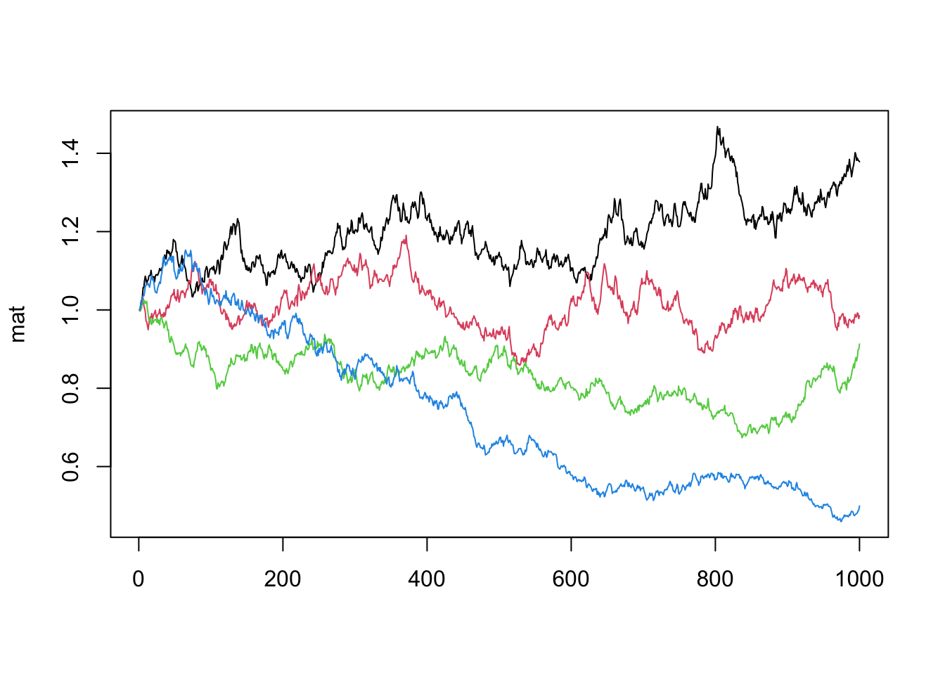
x = rnorm(N, mean = 0, sd = 0.01)
p = cumprod(x + 1)
p = p / p[1]
plot(p, type = 'l')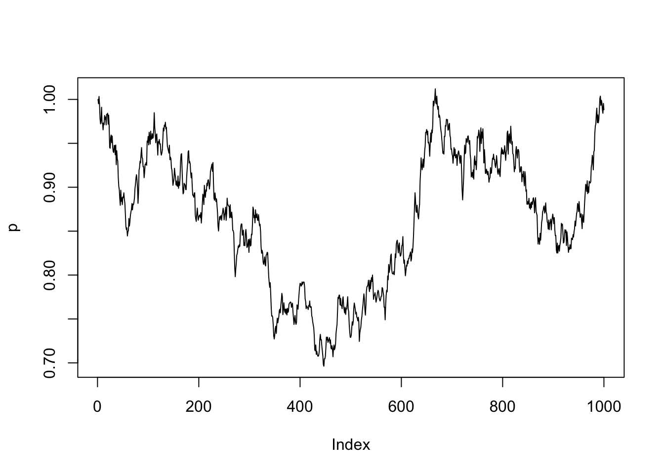
We can also do several random walks and plot them on the same figure.
N = 1000
R = 4
for(i in 1:R){
  p = cumprod(rnorm(N, mean = 1, sd = 0.01))
  p = p / p[1]
  if(i == 1){
    mat = p
  }else{
    mat = cbind(mat, p)
  }
}
matplot(mat, type = 'l', lty = 1)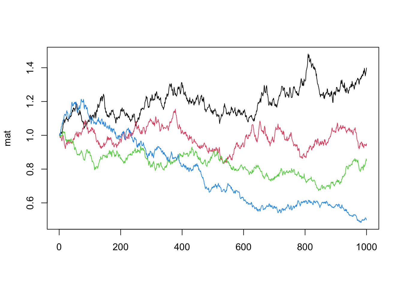
Random walks provide a foundation for more sophisticated financial applications. One of the most common uses of simulation in finance is option pricing, where analytical solutions may not exist or be computationally intensive.
13.6 Pricing options
It is very common to use simulations to price options. Below, we use it to price a standard Black-Scholes option. Of course, we know the true option price in that case, but that allows us to compare the accuracy of the simulation to the true value.
Start with a function for the Black-Scholes.
bs = function(X, P, r, sigma, T){
 d1 = (log(P/X) + (r + 0.5*sigma^2)*(T))/(sigma*sqrt(T))
 d2 = d1 - sigma*sqrt(T)
 Call = P*pnorm(d1, mean = 0, sd = 1) - X*exp(-r*(T))*pnorm(d2, mean = 0, sd = 1)
 Put = X*exp(-r*(T))*pnorm(-d2, mean = 0, sd = 1) - P*pnorm(-d1, mean = 0, sd = 1)
 Delta.Call = pnorm(d1, mean = 0, sd = 1)
 Delta.Put = Delta.Call - 1
 Gamma = dnorm(d1, mean = 0, sd = 1)/(P*sigma*sqrt(T))
 return(list(Call=Call,Put=Put,Delta.Call=Delta.Call,Delta.Put=Delta.Put,Gamma=Gamma))
}
And set some parameters for the option.
P0 = 50
sigma = 0.2
r = 0.05
T = 0.5
X = 40
bsprice = bs(X, P0, r, sigma, T)
print(bsprice)
$Call
[1] 11.08728
$Put
[1] 0.09967718
$Delta.Call
[1] 0.9660259
$Delta.Put
[1] -0.03397407
$Gamma
[1] 0.01066378We then create a function sim() that takes as arguments for the number of simulations, S and the seed.
sim = function(S = 1e6, seed = 666){
  set.seed(seed)
  F = P0 * exp(r * T)
  ysim = rnorm(S, -0.5 * sigma * sigma * T, sigma * sqrt(T))
  F = F * exp(ysim)
  SP = F - X
  SP[SP < 0] = 0
  fsim = SP * exp(-r * T)
  return(fsim)
}
Print ten simulations and plot a 100.
print(sim(S = 10)) [1] 16.054970 26.805763 8.065303 26.934463 0.000000 16.094585 2.140755
[8] 5.178977 0.000000 10.196711plot(sim(S = 100))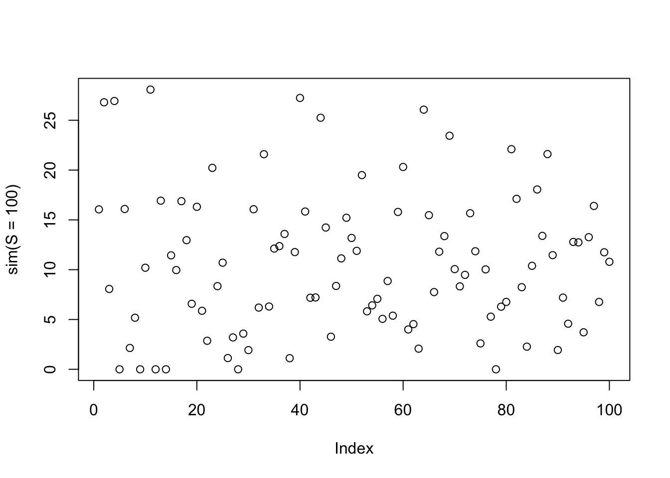
If we let the number of simulations vary over c(1e1,5e1,1e2,1e3,1e4), we can get a measurement of the accuracy of the number of simulations as their number increases:
cat("bs", bsprice$Call, "\n")bs 11.08728 for(S in c(1e1, 5e1, 1e2, 1e3, 1e4)){
cat(S, mean(sim(S = S)), "\n")
}10 11.14715
50 10.75441
100 10.65253
1000 10.93522
10000 11.19661 You could also use simulations to get the confidence bounds for the simulation estimates. We leave that as an exercise.
Below, we do a lot more simulations and plot their histogram with the superimposed true value.
fsim = sim()
hist(fsim,
  nclass = 100,
  probability = TRUE,
  xlim = c(0, 35),
  ylim = c(0, 0.12),
  col = 'red',
  las = 1,
  main = "",
  xlab = "Option prices",
  ylab = "Density"
)
segments(bsprice$Call, 0, bsprice$Call, 0.1, col = 'red')
text(bsprice$Call, 0.11, "Black-Scholes\nprice")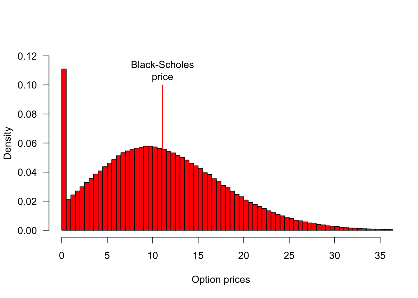
This example demonstrates the basic principles of Monte Carlo option pricing. For more sophisticated applications of simulation in risk management, including portfolio Value-at-Risk calculations and stress testing scenarios, see Chapter 21.
13.7 Multivariate
We sometimes need to simulate correlated values from a multivariate distribution, like we do in Chapter 21. The library MASS allows us to simulate multivariate normals, with mvrnorm.
mu = c(0, 0)
sigma = matrix(c(1, 0.8, 0.8, 1), ncol = 2)
data = mvrnorm(n = 1000, mu = mu, Sigma = sigma)
plot(data, col = "blue", pch = 16, main = "Multivariate Normal Simulation")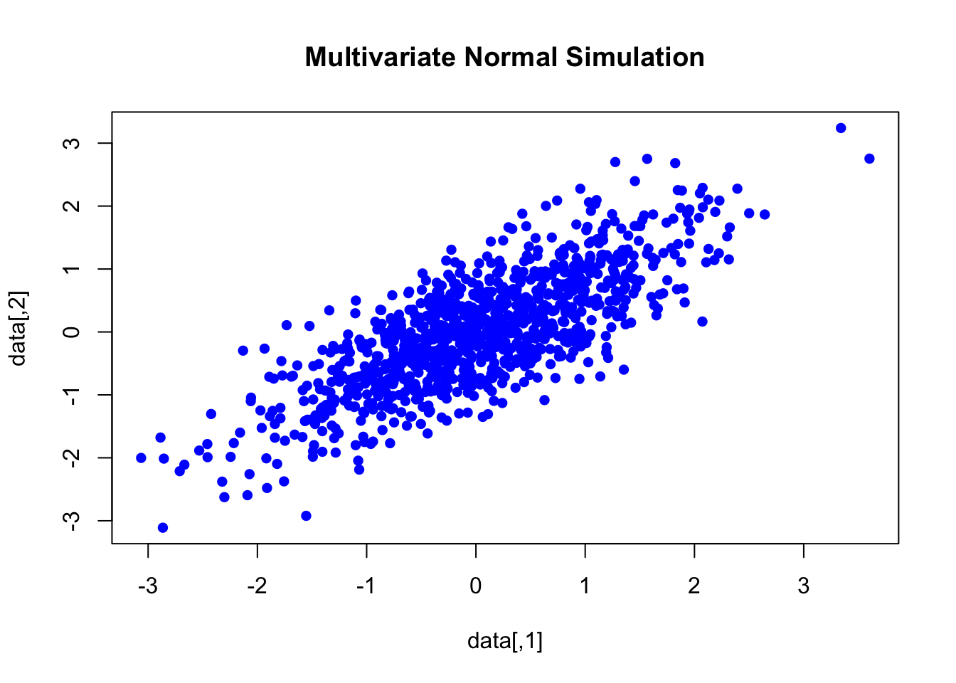
Library Copula can also be used.
normal_cop = normalCopula(param = 0.7, dim = 2)
sample = rCopula(1000, normal_cop)
plot(sample, col = "purple", pch = 16, main = "Gaussian Copula Simulation (uniform)")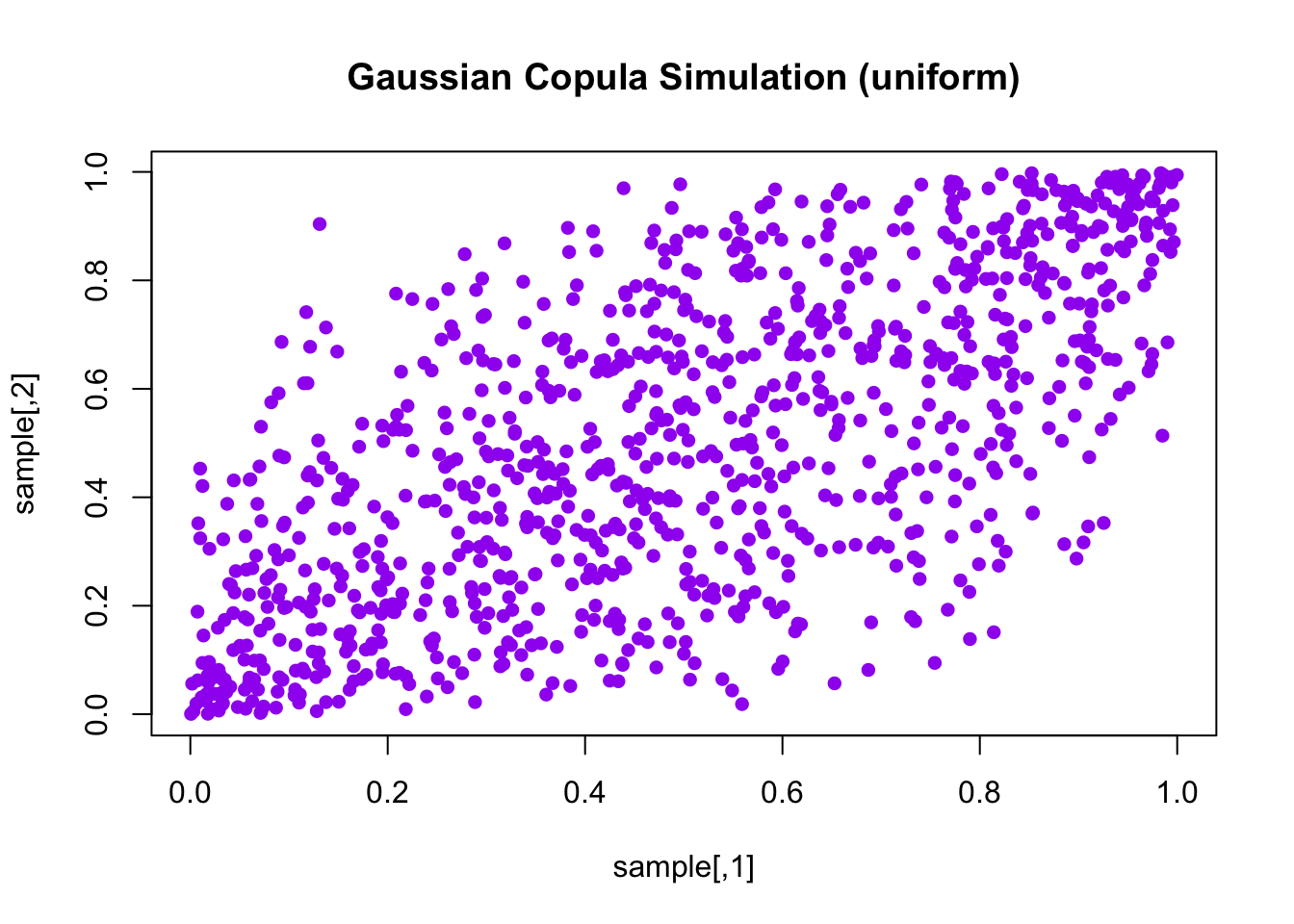
norm_samples = qnorm(sample)
plot(norm_samples, col = "purple", pch = 16, main = "Gaussian Copula Simulation (normal)")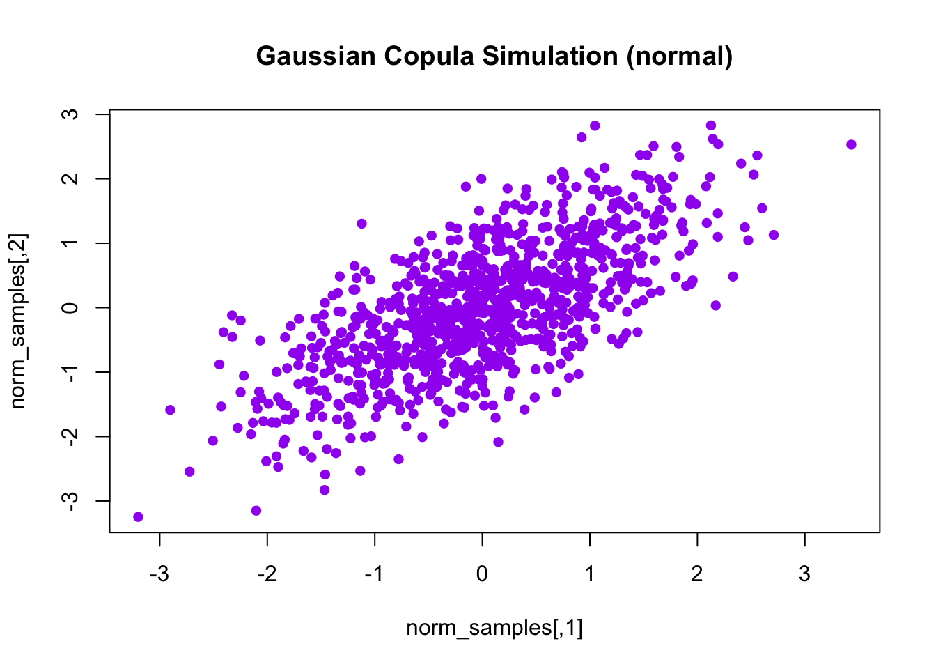
clayton_cop = claytonCopula(param = 2, dim = 2)
n_samples = 1000
u = rCopula(n_samples, clayton_cop)
plot(u, col = "blue", pch = 16,
     main = "Clayton Copula Simulation",
     xlab = "U1", ylab = "U2")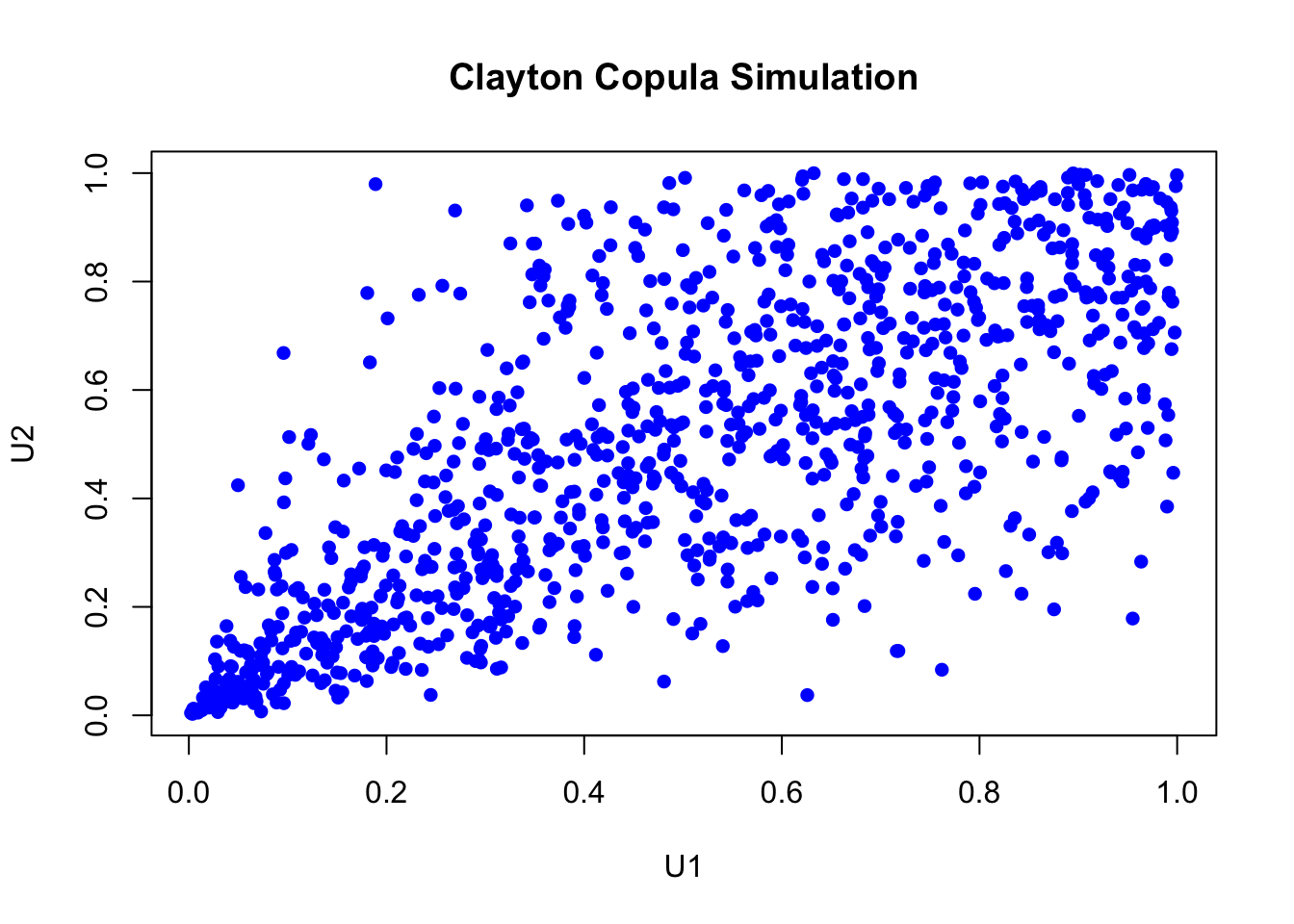
13.8 Exercise
Use simulations to get the confidence bounds for the simulation estimates.