21 Simulation methods for risk

While the analytical VaR methods from Chapter 20 work well for linear instruments like stocks and bonds, many financial instruments have non-linear payoffs that require simulation-based approaches. Simulation methods become necessary when:

Non-linear instruments: Options and other derivatives have payoffs that change non-linearly with underlying asset prices
Portfolio complexity: Multi-asset portfolios with derivatives cannot be evaluated using analytical formulas
Tail risk assessment: Simulation allows us to examine the full distribution of potential losses beyond normal distribution assumptions
Regulatory requirements: Basel framework requires advanced risk measurement for complex portfolios
Stress testing: Risk managers need to understand portfolio behaviour under extreme scenarios

Building on the VaR framework from Chapter 20 and the backtesting methods from Chapter 22, we now combine these approaches to handle complex instruments. The Monte Carlo techniques provide the foundation, while the VaR framework gives us the risk measurement structure.

For practitioners, simulation-based VaR is often the only feasible approach when portfolios contain derivatives, structured products, or when correlations become relevant under stress conditions.

The general approach follows these steps:

Set up simulation parameters and risk calculation framework
Simulate future asset prices or returns using appropriate stochastic processes
Calculate portfolio values under each simulation scenario
Compute profit/loss for each scenario
Extract VaR and ES from the simulated distribution

21.1 Data and libraries

We load the necessary packages for simulation-based risk analysis, including multivariate normal distribution functions.

library(mvtnorm)
source("common/functions.r",chdir=TRUE)

21.2 Black-Scholes equation

bs = function(K, P, r, sigma, T){
  d1 = (log(P/K) + (r + 0.5*sigma^2)*(T))/(sigma*sqrt(T))
  d2 = d1 - sigma*sqrt(T)
  Call = P*pnorm(d1) - K*exp(-r*(T))*pnorm(d2)
  Put = K*exp(-r*(T))*pnorm(-d2) - P*pnorm(-d1)
  return(list(Call=Call,Put=Put))
}

21.3 Simulating returns

It is worth noting that we are not pricing options and, therefore, do not have to worry about simulating prices under the risk-neutral distribution. We can use any stochastic process for returns we want and whichever definition of returns is most convenient.

In most of the examples below, we assume normality and use basic returns, but we could just as easily use any of the more complex models from Chapter 20, including those with non-normal conditional distributions and even historical simulation.

Simple returns are defined by \[ R_{t+1} = \frac{P_{t+1}}{P_t}-1 \] We know $P_t$ and simulate $R_{t+1}$ to get simulated price in the future $P_{t+1}$ so \[P_{t+1,s} = P_t \times (1+R_{t+1,s})\] where $s$ indicates a particular simulation.

Note $P_{t+1}$ is not the simulated futures price.

21.4 Number of assets

Portfolio simulation requires careful consideration of position sizes and asset weights. To build understanding systematically, we start with single-asset examples before extending to multi-asset portfolios.

In the examples below, we assume one holds one unit of each asset, which helps simplify the implementation. In that case, if one holds one stock, the current portfolio value is P. This assumption can easily be relaxed to handle arbitrary position sizes and portfolio weights.

21.5 One asset — Univariate

21.5.1 Setup

par = list()
par$probability = 0.05
par$S = 1e3
par$P = 100
par$r = 0.05
par$K = 99
par$Mat = 1
par$sigma = 0.01

21.5.2 Simulate prices

We create the function Sim.Prices(par) to implement the simulation. It takes the par list as an argument and returns a vector of simulated returns. If necessary, we could modify it to also return the Returns. It would also be straightforward to modify it to include other distributions besides the normal and even more advanced mean.

While S is already inside par, in some cases, we may want to input our own. For that purpose, we have a default argument, S=NULL, which does nothing. However, we can optionally input our own, which is then set by if(!is.null(S)) par$S=S. Also, we always set the seed, but if you do not want to, we can pass NULL as the seed.

Sim.Prices = function(par,seed=888,S=NULL){
    if(!is.null(seed)) set.seed(seed)
    if(!is.null(S)) par$S=S
    Returns = rnorm(
        n=par$S,
        mean=0,
        sd=par$sigma
    )
    Prices = par$P*(1+Returns)
    return(Prices)
}

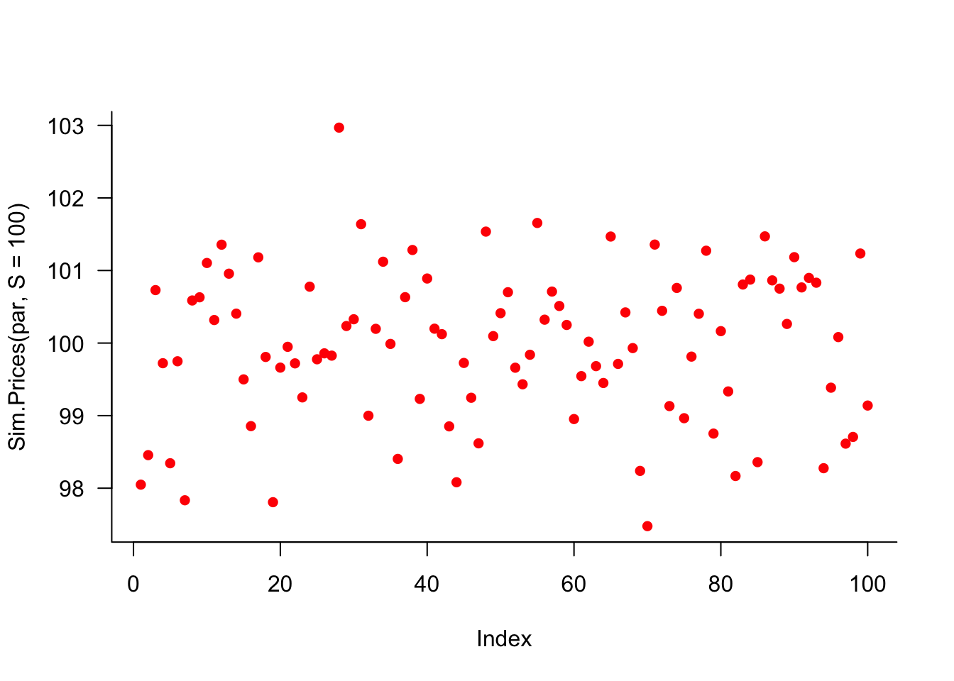
Here is one example.

plot(Sim.Prices(par,S=100),
    pch=16,
    col='red',
    las=1,
    bty='l'
)

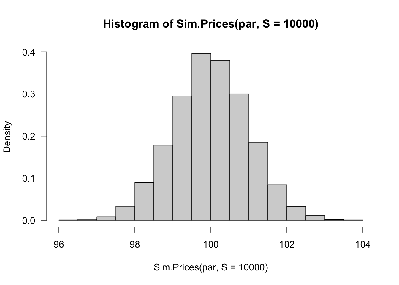
hist(
    Sim.Prices(par,S=10000),
    freq=FALSE,
    las=1
)

21.5.3 Design

The simulation-based VaR framework follows a consistent pattern across all examples. Understanding this general approach helps when extending to more complex portfolios and instruments.

The general setup below is that we first calculate the current portfolio value, called today, and then do the simulations to get the simulated vector of tomorrow’s portfolio value, called tomorrow. The difference between the two is profit and loss, PL. The VaR is then a quantile on the PL vector, while ES is the average from that quantile to the minimum.

21.5.4 VaR for one stock

cat("Number of simulations:",par$S,"\n")

Number of simulations: 1000

today = par$P
tomorrow = Sim.Prices(par,seed=8888)
PL = tomorrow - today
VaR = -sort(PL)[par$probability*par$S]
cat("VaR = $",VaR,"\n",sep="")

VaR = $1.808545

tomorrow = Sim.Prices(par,seed=666)
PL = tomorrow - today
VaR = -sort(PL)[par$probability*par$S]
cat("VaR = $",VaR,"\n",sep="")

VaR = $1.682279

We did two simulations with different seeds, and the two VaR numbers are quite different. We analyse the number of simulations below.

21.5.5 VaR for one option

When we have one option, we need to run the Black-Scholes equation for both today’s price and tomorrow’s simulated price.

x = Sim.Prices(par)
type = "Call"
today = bs(
    K=par$K,
    P=par$P,
    r=par$r,
    sigma=sqrt(250)*par$sigma,
    T=par$Mat
)[[type]]
tomorrow = bs(
    K=par$K,
    P=x,
    r=par$r,
    sigma=sqrt(250)*par$sigma,
    T=par$Mat-1/365
)[[type]]
PL = tomorrow - today
VaR = -sort(PL)[par$probability*par$S]
cat("VaR = $",VaR,"\n",sep="")

VaR = $1.094919

21.5.6 VaR for one stock and option

When we have one asset, and both hold it and have an option on it, we only simulate the prices once and use the same simulated price vector for both.

x = Sim.Prices(par)
type = "Call"
today = par$P
today =
    today+
    bs(
        K=par$K,
        P=par$P,
        r=par$r,
        sigma=sqrt(250)*par$sigma,
        T=par$Mat
    )[[type]]
tomorrow = x
tomorrow =
    tomorrow +
    bs(
        K=par$K,
        P=x,
        r=par$r,
        sigma=sqrt(250)*par$sigma,
        T=par$Mat-1/365
    )[[type]]
PL = tomorrow - today
VaR = -sort(PL)[par$probability*par$S]
cat("VaR = $",VaR,"\n",sep="")

VaR = $2.735947

21.6 Bivariate simulation

If we hold a portfolio of two stocks and options on each, we need to simulate from the bivariate normal distribution. In this case, we call rmvnorm(), but it would be straightforward to do it manually with a Choleski decomposition.

21.6.1 Setup

par = list()
par$probability = 0.05
par$S = 1e3
par$r = 0.05
par$P = c(100,25)
par$Sigma = rbind(
    c(0.01,0.005),
    c(0.005,0.02)
)
par$Mat = c(0.5,1)
par$K = c(90,30)

21.6.2 Simulate bivariate normal

It is then easy to use the number of simulations and the covariance matrix, par$Sigma, to simulate correlated returns and hence prices. Note that par$Sigma is the covariance matrix, while par$sigma is the standard deviation.

print(par$Sigma)

      [,1]  [,2]
[1,] 0.010 0.005
[2,] 0.005 0.020

r = rmvnorm(10,sigma=par$Sigma)
print(r)

              [,1]        [,2]
 [1,]  0.008934439 -0.15707369
 [2,] -0.089471235  0.07925927
 [3,]  0.076655490 -0.13516996
 [4,] -0.116082299 -0.10491110
 [5,] -0.096791561  0.02192440
 [6,]  0.016549428 -0.12714536
 [7,] -0.123844029  0.05159013
 [8,] -0.086154555 -0.14738669
 [9,] -0.152007705 -0.12858155
[10,] -0.004291241 -0.22524615

print(cov(r))

             [,1]         [,2]
[1,]  0.005652299 -0.003724937
[2,] -0.003724937  0.010262649

print(cor(r))

           [,1]       [,2]
[1,]  1.0000000 -0.4890764
[2,] -0.4890764  1.0000000

21.6.3 Simulate bivariate prices

Sim.BivarPrices = function(par,seed=666,S=NULL){
    if(!is.null(seed)) set.seed(seed)
    if(!is.null(S)) par$S=S
    Returns = rmvnorm(par$S,sigma=par$Sigma)
    Prices1 = par$P[1]*(1+Returns[,1])
    Prices2 = par$P[2]*(1+Returns[,2])
    return(cbind(Prices1,Prices2))
}

21.6.4 Two stocks

today = sum(par$P)
tomorrow = rowSums(Sim.BivarPrices(par))
PL = tomorrow - today
VaR = -sort(PL)[par$probability*par$S]
cat("VaR = $",VaR,"\n",sep="")

VaR = $18.59122

21.6.5 Two stocks and two options

21.6.5.1 Today

type = c("Call","Put")
today = sum(par$P)
for(i in 1:2){
    today = today +
        bs(
            K=par$K[i],
            P=par$P[i],
            r=par$r,
            sigma=sqrt(250)*sqrt(par$Sigma[i,i]),
            T=par$Mat[i]
        )[[type[i]]]
}

21.6.5.2 Tomorrow

x=Sim.BivarPrices(par)
tomorrow = 0
for(i in 1:2){
    tomorrow = tomorrow +
        x[,i] +
        bs(
            K=par$K[i],
            P=x[,i],
            r=par$r,
            sigma=sqrt(250)*sqrt(par$Sigma[i,i]),
            T=par$Mat[i]-1/365
        )[[type[i]]]
}
PL = tomorrow - today
VaR=-sort(PL)[par$probability*par$S]
cat("VaR = $",VaR,"\n",sep="")

VaR = $30.02989

21.7 Sim VaR vs. true VaR

Since we know the true VaR in cases where we do not have the option, we can easily compare the true number to the one obtained by simulations. As the number of simulations increases, these two values should converge. And if they do not, we have done something wrong. We can also use this to ascertain how many simulations we need.

21.7.1 Setup

par = list()
par$probability = 0.01
par$P = 100
par$sigma = 0.01

21.7.2 VaR for one stock

To facilitate the analysis, we create a function simVaR() that returns simulated VaR. Because it allows us to vary the seed number of simulations, we can get an idea of the accuracy.

simVaR = function(par,S,seed=14){
    set.seed(seed)
    today = par$P
    par$S = S
    tomorrow = Sim.Prices(par,seed=seed)
    PL = tomorrow - par$P
    VaR = -sort(PL)[par$probability*par$S]
    return(VaR)
}

Here, we show the simulated and true VaR.

VaR = simVaR(par=par,S=100)
cat("VaR = $",VaR,"\n",sep="")

VaR = $2.136976

trueVaR = - par$P * qnorm(par$probability) * par$sigma
cat("trueVaR = $",trueVaR,"\n",sep="")

trueVaR = $2.326348

We can repeat this:

trueVaR = - par$P * qnorm(par$probability) * par$sigma
N = 10
VaR = vector(length=10)
for(i in 1:N) VaR[i] = simVaR(par=par,S=100,seed=i)
Error = VaR - trueVaR
True = 0*VaR + trueVaR
df = as.data.frame(cbind(True,VaR,Error))
print(df)

       True      VaR      Error
1  2.326348 2.214700 -0.1116480
2  2.326348 2.451706  0.1253585
3  2.326348 2.265401 -0.0609468
4  2.326348 1.797382 -0.5289659
5  2.326348 2.183967 -0.1423811
6  2.326348 1.952349 -0.3739992
7  2.326348 1.785893 -0.5404544
8  2.326348 3.014527  0.6881794
9  2.326348 2.617706  0.2913577
10 2.326348 2.185287 -0.1410610

We can also vary the number of simulations.

S = c(1e3,1e4,1e5,1e6,1e7)
VaR = S
for(i in 1:length(S)) VaR[i] = simVaR(par=par,S=S[i])
df = as.data.frame(cbind(S,VaR))
df$error = df$VaR - trueVaR
print(df)

      S      VaR         error
1 1e+03 2.327881  0.0015331722
2 1e+04 2.392073  0.0657246966
3 1e+05 2.315741 -0.0106066797
4 1e+06 2.325955 -0.0003930874
5 1e+07 2.326765  0.0004172930

S = c(seq(1e4,1e4,by=100),seq(1e4,1e6,by=1000))
VaR = S
for(i in 1:length(S)) VaR[i] = simVaR(par=par,S=S[i])
df = as.data.frame(cbind(S,VaR))
df$error = df$VaR - trueVaR
plot(
    df[,1],df[,2],
    type='l',
    lty=1,
    col="red",
    bty='l',
    las=1,
    xlab="simulations",
    ylab="VaR")
segments(min(S),trueVaR,max(S),trueVaR,col="blue",lwd=3)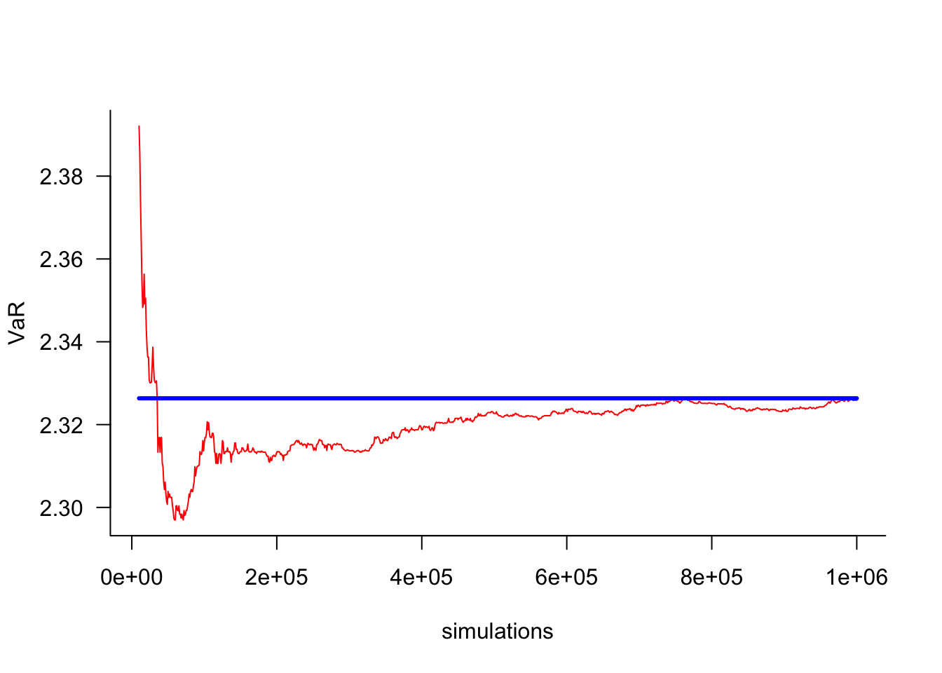

21.8 Extensions

The simulation framework presented here can be extended in several directions to handle more realistic portfolio situations. These extensions demonstrate the flexibility of simulation-based approaches compared to analytical methods.

Possible extensions include:

Variable number of assets: Scaling the framework to handle portfolios with dozens or hundreds of underlying assets
Complex derivative positions: Holding multiple options on each stock, with puts and calls, a range of strikes and maturities
Realistic position sizes: Moving beyond unit holdings to handle actual portfolio weights and position sizes
Advanced stochastic processes: Incorporating GARCH volatility models, jump processes, or regime-switching behaviour from the models in Chapter 20

These extensions maintain the same basic simulation structure whilst accommodating the complexity found in real-world portfolios.

21.9 Exercise

Make a function that allows an arbitrarily sized number of assets
Reimplement the examples above using historical simulation
Use GARCH(1,1) to obtain time-varying volatilities and implement backtesting