source("common/functions.r",chdir=TRUE)
library(rugarch)
library(lubridate)
library(reshape2)16 Univariate volatility
Univariate volatility modelling is designed to provide an in-sample description of the stochastic processes governing volatility. More importantly, for our purpose here, it also gives one-day-ahead volatility forecasts, which we use for risk calculations.
The mathematics of univariate volatility models are discussed in Chapter 2 of Financial Risk Forecasting.
We use maximum likelihood methods for estimating volatility models and use the R package rugarch for the actual implementation. See the package documentation for more details and a more detailed vignette. It is developed by Alexios Galanos and is regularly maintained and updated. The development code can be found on GitHub.
The developer of rugarch, Alexios Galanos, has released an updated volatility package called tsgarch, suggesting users should use that instead. The reason we still use the older rugarch here is because the multivariate versions of tsgarch were released quite recently, and there are still some issues with installing the necessary support libraries for that. Once that stabilises, we will switch.
This chapter uses a long data sample, and all the estimation works without problems. In Chapter 17, we will see what can go wrong with volatility models and how to fix them.
16.1 Data and libraries
data=ProcessRawData()
y=data$sp500$y
y=y-mean(y)
16.1.1 What to do with the mean?
One should either remove the mean — de-mean — of the returns or estimate it along with the other parameters. We can also forecast the mean along with volatility, as shown below.
However, since the mean is quite small, we can usually ignore it if the sample size is large. Chapter 17 shows how that can fail.
16.2 EWMA
The exponentially weighted moving average (EWMA) model provides a simple approach to volatility forecasting that assigns exponentially declining weights to past observations. Unlike more complex GARCH models, EWMA requires only one parameter (\(\lambda\)) and is computationally straightforward, making it a useful benchmark for comparison.
The EWMA volatility forecast is given by:
\[\sigma_t^2 = \lambda \sigma_{t-1}^2 + (1-\lambda) y_{t-1}^2\]
where \(\sigma_t^2\) is the conditional variance at time \(t\), \(y_{t-1}\) is the return at time \(t-1\), and \(\lambda\) is the decay parameter (typically around 0.94 for daily data).
We estimate the in-sample EWMA volatility and plot the returns with ±2 standard deviation bands.
EWMA = vector(length=length(y))
lambda = 0.94
EWMA[1] = var(y)
for (i in 2:length(y)){
    EWMA[i] =
        lambda * EWMA[i-1]+
        (1-lambda) * y[i-1] ^2
}
EWMA=sqrt(EWMA)

par(mar=c(2,3.5,1,0))
matplot(
 cbind(y,2*EWMA,-2*EWMA),
 type='l',
 lty=1,
 col=c("black","red","red"),
 bty='l',
 ylab="",
 main="S&P 500 returns with ±2 EWMA sd",
 las=1
)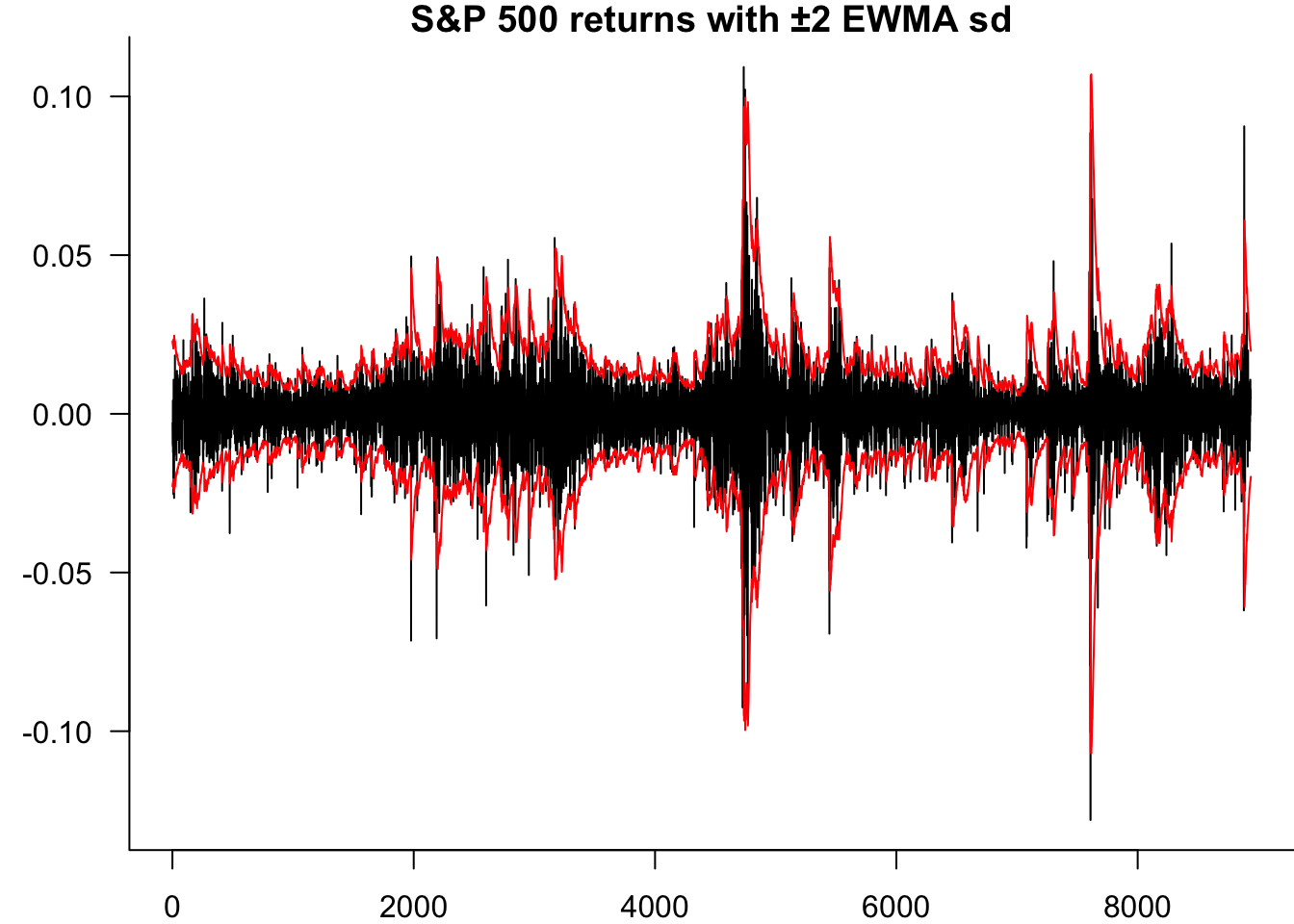
While EWMA provides a useful baseline, it has limitations including the inability to capture volatility clustering patterns and the restriction to a single parameter. GARCH models address these limitations by allowing for more flexible lag structures and distributional assumptions.
16.3 GARCH
GARCH models provide a flexible framework for capturing the time-varying volatility observed in financial time series. These models allow volatility to depend on past volatility (the GARCH component) and past squared returns (the ARCH component), whilst accommodating different distributional assumptions for the innovations.
We implement GARCH models using the rugarch package, which provides comprehensive tools for specification, estimation and forecasting. The package supports various GARCH variants including asymmetric models that capture the leverage effect common in equity returns.
16.3.1 Setup
The rugarch package uses an object-oriented approach that separates model specification from estimation. This design allows you to define multiple model configurations and apply them to different datasets without repetition. The workflow is deliberately structured to encourage good practice: first think carefully about your model specification, then estimate.
This two-step process also facilitates model comparison, as you can easily modify specifications and re-estimate without changing the underlying code structure.
To estimate a univariate GARCH model with rugarch, we need to follow two steps:
- Create an object of the
uGARCHspecclass, which is the specification of the model you want to estimate. This includes the type of model (standard, asymmetric, power, etc.), the GARCH order, the distribution, and the model for the mean; - Fit the specified model to the data.
16.3.2 ugarchspec()
The ugarchspec() function creates model definitions in rugarch. It specifies the volatility dynamics, mean equation, and distributional assumptions for your GARCH model.
Understanding this function is useful because it controls the key aspects of your model. Proper specification helps achieve reliable estimates, whilst poor specification can lead to convergence issues or unreliable results.
First let us take a look at ugarchspec(), which is the function to create an instance of the uGARCHspec class. The complete syntax with its default values is:
ugarchspec(
 variance.model = list(
    model = "sGARCH",
    garchOrder = c(1, 1),
    submodel = NULL,
    external.regressors = NULL,
    variance.targeting = FALSE
    ),
 mean.model = list(
    armaOrder = c(1, 1),
    include.mean = TRUE,
    archm = FALSE,
    archpow = 1,
    arfima = FALSE,
    external.regressors = NULL,
    archex = FALSE
 ),
 distribution.model = "norm",
 start.pars = list(),
 fixed.pars = list()
 )
*---------------------------------*
*       GARCH Model Spec          *
*---------------------------------*

Conditional Variance Dynamics
------------------------------------
GARCH Model     : sGARCH(1,1)
Variance Targeting  : FALSE

Conditional Mean Dynamics
------------------------------------
Mean Model      : ARFIMA(1,0,1)
Include Mean        : TRUE
GARCH-in-Mean       : FALSE

Conditional Distribution
------------------------------------
Distribution    :  norm
Includes Skew   :  FALSE
Includes Shape  :  FALSE
Includes Lambda :  FALSE
You can check the details of this function and what every argument means by running ?ugarchspec.
For the purposes of our course, we are going to focus on three arguments of the ugarchspec() function:
16.3.2.1 variance.model
The variance.model argument defines how volatility evolves over time. This is where you specify the fundamental structure of your volatility process, including which GARCH variant to use and how many lags to include.
This argument takes a list with the specifications of the GARCH model. Its most important components are:
model: Specify the type of model. Currently implemented models are “sGARCH”, “fGARCH”, “eGARCH”, “gjrGARCH”, “apARCH”, “iGARCH”, and “csGARCH”garchOrder: Specify the ARCH(q) and GARCH(p) orders
Other components include options to do variance.targeting or external regressors.
16.3.2.2 mean.model
The mean.model argument specifies how the expected return evolves over time. This includes whether to estimate a constant mean and any autoregressive or moving average components.
This argument takes a list with the specifications of the mean model and is assumed to have one. A traditional assumption is that the model has zero mean, in which case we specify armaOrder = c(0,0), include.mean = FALSE. However, it is also common to assume that the mean follows a certain ARMA process.
16.3.2.3 distribution.model
The distribution.model argument determines the probability distribution assumed for the standardised residuals. This choice affects tail behaviour and the likelihood of extreme observations.
Here, we can specify the conditional density to use for innovations. The default is a normal distribution, but we can specify some others, perhaps the Student-t distribution std, or the asymmetric Student-t distribution sstd.
16.3.3 ugarchfit()
The ugarchfit() function performs the actual parameter estimation using the model specification you have created. It applies maximum likelihood estimation to find the parameter values that best fit your data.
Once the specification has been created, you can fit this to the data using ugarchfit( spec = ..., data = ...). The result will be an object of the class uGARCHfit, which is a list that contains useful information, as shown below.
16.3.4 Optimiser failure — Hybrid
Maximum likelihood estimation for GARCH models involves finding parameter values that maximise a complex, non-linear likelihood function. This optimisation can be challenging because the likelihood surface may have multiple local maxima, flat regions, or numerical instabilities.
The rugarch package uses numerical optimisation algorithms (solvers) to find the maximum likelihood estimates. The default solver works well in most cases, but complex models or difficult datasets can cause convergence failures. Common issues include starting values that are too far from the optimum, boundary constraints that restrict the search space, or numerical precision problems. See discussion in Section 18.2.
The solver = "hybrid" option addresses these challenges by sequentially trying multiple optimisation algorithms. If the first method fails, it automatically switches to alternative approaches with different strengths. This increases the likelihood of finding a solution, though it may take longer to compute.
16.4 The models
Having covered the theoretical framework and software mechanics, we now estimate a range of GARCH model variants to demonstrate their practical implementation. Each model captures different aspects of volatility dynamics: symmetric versus asymmetric responses to shocks, normal versus heavy-tailed distributions, and constant versus time-varying means.
We estimate eight different specifications to illustrate the flexibility of the GARCH framework. These range from simple ARCH models to complex asymmetric specifications with non-normal distributions. This variety allows us to compare model performance and understand how different assumptions affect the results.
We will put the results into a list called Results so we can automatically process them afterwards.
Results=list()16.4.1 Gaussian ARCH(1) and no mean
We start with the simplest volatility model: ARCH(1) with Gaussian innovations and no mean equation. This model assumes volatility depends only on the previous period’s squared return, providing a baseline for comparison with more complex specifications.
The garchOrder in variance.model will be set as c(1,0). Note that even if we only have one component, we need to put it inside a list.
spec.1 = ugarchspec(
 variance.model = list(
 garchOrder = c(1,0)
 ),
 mean.model = list(
 armaOrder = c(0,0),
 include.mean = FALSE
 )
)
We can call spec.1 to see what is inside:
spec.1
*---------------------------------*
*       GARCH Model Spec          *
*---------------------------------*

Conditional Variance Dynamics
------------------------------------
GARCH Model     : sGARCH(1,0)
Variance Targeting  : FALSE

Conditional Mean Dynamics
------------------------------------
Mean Model      : ARFIMA(0,0,0)
Include Mean        : FALSE
GARCH-in-Mean       : FALSE

Conditional Distribution
------------------------------------
Distribution    :  norm
Includes Skew   :  FALSE
Includes Shape  :  FALSE
Includes Lambda :  FALSE
Now we can fit the specified model to our data using the ugarchfit() function:
Results$ARCH1 = ugarchfit(spec = spec.1, data = y)That can fails and we may need the hybrid solver.
Results$ARCH1 = ugarchfit(spec = spec.1, data = y,solver = "hybrid")We can check the class of this new object:
class(Results$ARCH1)[1] "uGARCHfit"
attr(,"package")
[1] "rugarch"16.4.1.0.1 Printing and plotting
To get all the results, use print(Results$ARCH1) and plot(Results$ARCH1).
Objects from the uGARCHfit class have two slots (an R term for an object of what is known as the S4). You can think of every slot as a list of components. The two slots are:
@model;@fit.
To access a slot, you need to use the syntax: object@slot
16.4.1.0.2 @model
The @model slot includes all the information that was needed to estimate the GARCH model. This includes both the model specification and the data. To see everything that is included in this slot, you can use the names() function:
names(Results$ARCH1@model) [1] "modelinc" "modeldesc" "modeldata" "pars" "start.pars"
[6] "fixed.pars" "maxOrder" "pos.matrix" "fmodel" "pidx"
[11] "n.start" And you can access each element with the $ sign. For example, let us see what is inside pars (only rows 7-10).
Results$ARCH1@model$pars[7:10,] Level Fixed Include Estimate LB UB
omega 8.530334e-05 0 1 1 2.220446e-16 0.1308107
alpha1 3.701577e-01 0 1 1 0.000000e+00 1.0000000
beta 0.000000e+00 0 0 0 NA NA
gamma 0.000000e+00 0 0 0 NA NAWe have a matrix with all the possible parameters for fitting a GARCH model. The parameters included in our GARCH specification (omega, alpha1, and beta1) have a value of 1. The matrix also includes the lower and upper bounds for these parameters, which have nothing to do with our particular data but with what is expected from the model.
We can also see the model description:
Results$ARCH1@model$modeldesc$distribution
[1] "norm"
$distno
[1] 1
$vmodel
[1] "sGARCH"Inside Results$ARCH1@model$modeldata, we will find the data vector we used when fitting the model. The @model slot contains everything that R needs to know to estimate the model.
16.4.1.0.3 @fit
Inside the fit slot, we will find the estimated model, including the coefficients, likelihood, fitted conditional variance, and more. Let us check everything that is included:
names(Results$ARCH1@fit) [1] "hessian" "cvar" "var" "sigma"
[5] "condH" "z" "LLH" "log.likelihoods"
[9] "residuals" "coef" "robust.cvar" "A"
[13] "B" "scores" "se.coef" "tval"
[17] "matcoef" "robust.se.coef" "robust.tval" "robust.matcoef"
[21] "fitted.values" "convergence" "kappa" "persistence"
[25] "timer" "ipars" "solver" Let us see the coefficients, along with their standard errors, in matcoef. There are two ways to do that:
Results$ARCH1@fit$matcoef Estimate Std. Error t value Pr(>|t|)
omega 8.530334e-05 1.768188e-06 48.24336 0
alpha1 3.701577e-01 2.236925e-02 16.54762 0coef(Results$ARCH1) omega alpha1
8.530334e-05 3.701577e-01 We can also see the log-likelihood. Again, there are two ways:
Results$ARCH1@fit$LLH[1] 27908.47likelihood(Results$ARCH1)[1] 27908.47This makes it easy to extract the estimated conditional volatility:
plot(Results$ARCH1@fit$sigma, type = "l")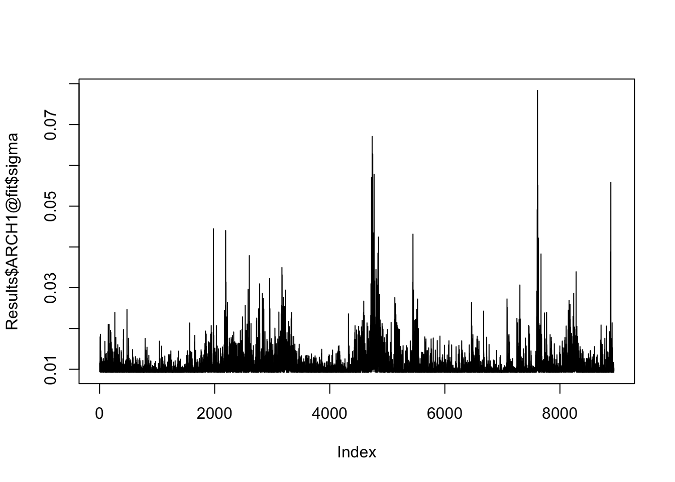
16.4.2 Gaussian GARCH(1,1)
The GARCH(1,1) model extends ARCH by including lagged volatility terms. This creates persistence in volatility clustering, a key feature of financial time series where periods of high volatility tend to be followed by more high volatility.
spec.2 = ugarchspec(
 variance.model = list(garchOrder = c(1,1)),
 mean.model = list(armaOrder = c(0,0), include.mean = FALSE)
)
Results$GARCH11 = ugarchfit(spec = spec.2, data = y,solver = "hybrid")
Results$GARCH11@fit$matcoef
Estimate Std. Error t value Pr(>|t|)
omega 8.021918e-08 2.466224e-07 0.3252712 0.7449758
alpha1 7.673806e-02 5.284567e-03 14.5211634 0.0000000
beta1 9.297933e-01 4.717754e-03 197.0838792 0.000000016.4.3 tGARCH(1,1)
We now allow for heavier tails by using Student-t distributed innovations instead of normal. This better captures the extreme returns commonly observed in financial markets whilst maintaining the same volatility dynamics.
We can see that the coefficients now include shape, which is the estimated degrees of freedom:
spec.3 = ugarchspec(
 variance.model = list(garchOrder = c(1,1)),
 mean.model = list(armaOrder = c(0,0), include.mean = FALSE),
 distribution.model = "std"
)
Results$tGARCH11 = ugarchfit(spec = spec.3, data = y,solver = "hybrid")
Results$tGARCH11@fit$matcoef
Estimate Std. Error t value Pr(>|t|)
omega 1.162910e-06 6.494341e-07 1.790651 0.07334935
alpha1 1.000315e-01 1.108772e-02 9.021830 0.00000000
beta1 8.946775e-01 1.035658e-02 86.387326 0.00000000
shape 6.311630e+00 3.241513e-01 19.471250 0.0000000016.4.4 Asymmetric tGARCH(1,1)
The skewed Student-t distribution accommodates both heavy tails and asymmetry in the return distribution. This allows the model to capture the negative skewness often found in equity returns.
We can have a skew Student-t conditional distribution.
spec.4 = ugarchspec(
 variance.model = list(garchOrder = c(1,1)),
 mean.model = list(armaOrder = c(0,0), include.mean = FALSE),
 distribution.model = "sstd"
)
Results$atGARCH11 = ugarchfit(spec = spec.4, data = y,solver = "hybrid")
Results$atGARCH11@fit$matcoef
Estimate Std. Error t value Pr(>|t|)
omega 1.185012e-06 6.986140e-07 1.696233 0.08984183
alpha1 1.003697e-01 1.178511e-02 8.516654 0.00000000
beta1 8.936189e-01 1.111000e-02 80.433747 0.00000000
skew 9.021712e-01 1.205819e-02 74.818157 0.00000000
shape 6.640385e+00 3.384229e-01 19.621558 0.0000000016.4.5 Gaussian apARCH model
The apARCH specification introduces asymmetric volatility responses, where negative returns can have different impacts on future volatility than positive returns of the same magnitude. This captures the leverage effect common in equity markets.
The parameter list will now include gamma1 and delta, which are part of the apARCH model specification:
spec.5 = ugarchspec(
 variance.model = list(model = "apARCH"),
 mean.model = list(armaOrder = c(0,0), include.mean = FALSE),
)

Results$APGARCH11 = ugarchfit(spec = spec.5, data = y,solver = "hybrid")
Results$APGARCH11@fit$matcoef
Estimate Std. Error t value Pr(>|t|)
omega 1.368453e-07 2.273019e-07 0.6020421 5.471461e-01
alpha1 5.000238e-02 1.059206e-02 4.7207428 2.349849e-06
beta1 8.895480e-01 1.239125e-02 71.7883891 0.000000e+00
gamma1 5.039665e-01 8.519092e-02 5.9157298 3.304072e-09
delta 2.534182e+00 2.647964e-02 95.7030337 0.000000e+0016.4.6 t-apARCH model
Combining asymmetric volatility dynamics with heavy-tailed innovations provides a more realistic representation of equity return behaviour.
spec.6 = ugarchspec(
 variance.model = list(model = "apARCH"),
 mean.model = list(armaOrder = c(0,0), include.mean = FALSE),
 distribution.model = "std"
)
Results$tAPGARCH11 = ugarchfit(spec = spec.6, data = y,solver = "hybrid")
Results$tAPGARCH11@fit$matcoef
Estimate Std. Error t value Pr(>|t|)
omega 2.282256e-08 2.028305e-06 0.01125203 9.910224e-01
alpha1 8.895176e-02 1.450010e-02 6.13456338 8.539340e-10
beta1 9.312873e-01 1.312771e-02 70.94057029 0.000000e+00
gamma1 5.595887e-01 1.027967e-01 5.44364372 5.220158e-08
delta 1.293171e+00 1.845368e-01 7.00765652 2.423395e-12
shape 5.934863e+00 3.650238e-01 16.25883914 0.000000e+0016.4.7 Asymmetric t-apARCH model
This specification combines all three extensions: asymmetric volatility, heavy tails, and return distribution skewness.
spec.7 = ugarchspec(
 variance.model = list(model = "apARCH"),
 mean.model = list(armaOrder = c(0,0), include.mean = FALSE),
 distribution.model = "sstd"
)
Results$atAPGARCH11 = ugarchfit(spec = spec.7, data = y,solver = "hybrid")
Results$atAPGARCH11@fit$matcoef
Estimate Std. Error t value Pr(>|t|)
omega 2.179889e-08 1.909960e-06 0.01141327 9.908937e-01
alpha1 8.937075e-02 1.211916e-02 7.37433665 1.652012e-13
beta1 9.305799e-01 1.077796e-02 86.34096632 0.000000e+00
gamma1 5.546509e-01 8.555606e-02 6.48289409 8.997958e-11
delta 1.304569e+00 1.525320e-01 8.55275781 0.000000e+00
skew 9.001966e-01 1.234568e-02 72.91590535 0.000000e+00
shape 6.174613e+00 3.986531e-01 15.48868793 0.000000e+0016.4.8 Asymmetric t-apARCH model with ARMA(1,1) mean
Our most complex specification adds a time-varying mean structure to capture potential predictability in returns alongside the sophisticated volatility and distributional assumptions.
spec.8 = ugarchspec(
 variance.model = list(model = "apARCH"),
 mean.model = list(armaOrder = c(1,1), include.mean = TRUE),
 distribution.model = "sstd"
)
Results$Mean.atAPGARCH11 = ugarchfit(spec = spec.8, data = y,solver = "hybrid")
Results$Mean.atAPGARCH11@fit$matcoef
Estimate Std. Error t value Pr(>|t|)
mu 1.403034e-16 7.344677e-05 1.910273e-12 1.000000e+00
ar1 6.246253e-01 7.345890e-02 8.503058e+00 0.000000e+00
ma1 -6.643195e-01 7.097233e-02 -9.360261e+00 0.000000e+00
omega 2.384660e-08 1.233822e-06 1.932743e-02 9.845799e-01
alpha1 8.811255e-02 1.228986e-02 7.169535e+00 7.525092e-13
beta1 9.317661e-01 1.039457e-02 8.963969e+01 0.000000e+00
gamma1 4.778694e-01 7.115285e-02 6.716097e+00 1.866574e-11
delta 1.340077e+00 1.229854e-01 1.089623e+01 0.000000e+00
skew 8.873079e-01 1.283753e-02 6.911829e+01 0.000000e+00
shape 6.113152e+00 3.941981e-01 1.550782e+01 0.000000e+0016.5 Comparing results
Having estimated eight different GARCH specifications, we now organise the results for systematic comparison. By consolidating the key statistics into a single data frame, we can easily compare log-likelihoods, parameter estimates, and computation times across models. This structured approach facilitates model selection and helps identify which specifications provide the best fit to our data.
We can put all the results into a dataframe
r=Results[[length(Results)]]

df=data.frame(c(likelihood(r),r@fit$timer,coef(r)))
rownames(df)[1:2]=c("log.likelihood","time")
rownames(df)[3:dim(df)[1]]=names(coef(r))
names(df)=names(Results)[length(Results)]


for(i in 1:length(Results)){
 r=Results[[i]]
 x=c(likelihood(r),r@fit$timer,coef(r))
   if(! is.null(likelihood(r))){
    x=data.frame(c(likelihood(r),r@fit$timer,coef(r)))
    rownames(x)[1:2]=c("log.likelihood","time")
    rownames(x)[3:dim(x)[1]]=names(coef(r))

    df[[names(Results)[i]]]=NA
    df[rownames(x),names(Results)[i]]=x
   }
}
df=round(df,3)
df=df[,names(Results)]

df.summary=df
16.5.1 Sample size considerations
It is worth considering that the more parameters a model has, the more it may run into estimation problems and the more data we need. Complex models require larger samples to achieve reliable parameter estimates and stable convergence.
For example, as a rule of thumb, for a GARCH(1,1), we need at least 500 observations, while for a Student-t GARCH, that minimum number can be around 3,000 observations. Asymmetric models with skewed distributions may require even larger samples due to their additional parameters.
In general, the more parameters are estimated, the more data is needed to be confident in the estimation. Insufficient sample sizes can lead to parameter instability, convergence failures, or unreliable standard errors. We see an example of this in Chapter 17.
16.6 Diagnostics
Model estimation is only the first step in statistical analysis. We must validate our fitted models to ensure they adequately capture the data characteristics and that our parameter estimates are reliable. Diagnostic testing helps identify model misspecification and guides the selection process among competing specifications.
16.6.1 Likelihood ratio test
The likelihood ratio test provides a formal framework for comparing nested models. By testing whether additional parameters significantly improve the model fit, we can determine if increased complexity is justified by the data.
The likelihood ratio (LR) test compares two models based on the ratio of their likelihoods,
# Perform the LR test
LR_statistic = 2*(likelihood(Results$GARCH11)-likelihood(Results$ARCH1))
p_value = 1 - pchisq(LR_statistic, df = 1)

cat(" Likelihood of ARCH: ", round(likelihood(Results$ARCH1),1), "\n",
 "Likelihood of GARCH:", round(likelihood(Results$GARCH11),1), "\n",
 "2 * (Lu - Lr): ", round(LR_statistic,2), "\n",
 "p-value:", p_value)
Likelihood of ARCH: 27908.5
Likelihood of GARCH: 29156.8
2 * (Lu - Lr): 2496.56
p-value: 0We find a p-value of 0, meaning that we have enough evidence to reject the null hypothesis that the two models are the same. The GARCH model has a significantly larger likelihood than the ARCH model.
16.6.2 Residual analysis
Examining standardised residuals reveals whether our model successfully captures the volatility dynamics. Unlike price forecasting where we can directly compare predictions with observed outcomes, volatility is latent and unobservable. We can only validate our volatility models indirectly through residual behaviour. Well-specified models should produce residuals that are approximately independent and identically distributed, with no remaining volatility clustering.
16.6.2.1 GARCH
We analyse the standardised residuals from our GARCH(1,1) model to check for remaining serial correlation and distributional assumptions. Any patterns in these residuals suggest areas where the model specification might be improved.
residuals=y/Results$GARCH11@fit$sigma
par(mar=c(2,4,2,0))
plot(residuals,type='l',bty='l',las=1)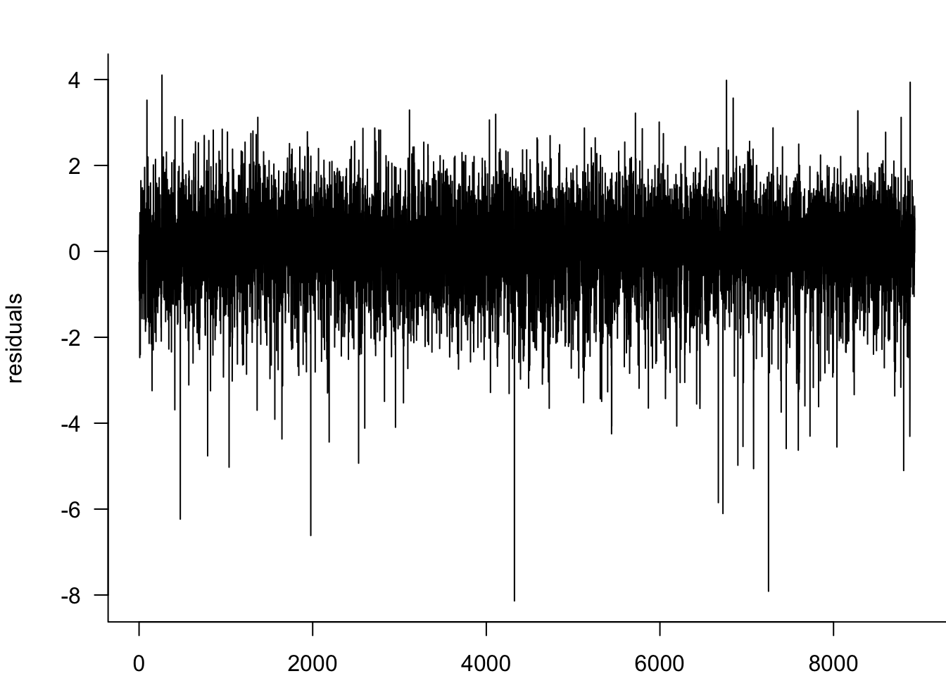
myACF(residuals,main="ACF of S&P 500 returns")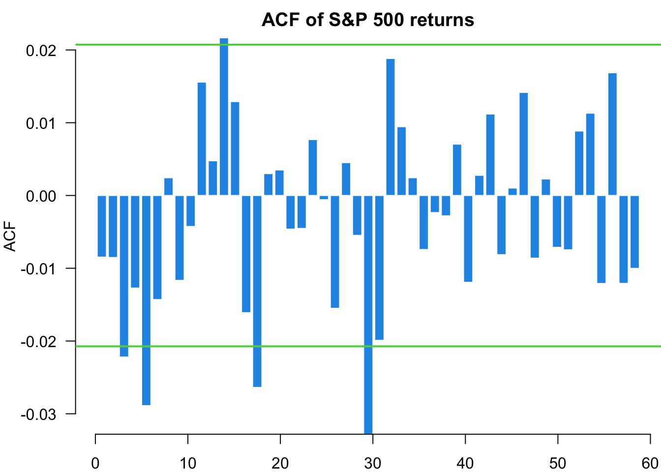
myACF(residuals^2,main="ACF of squared S&P 500 returns")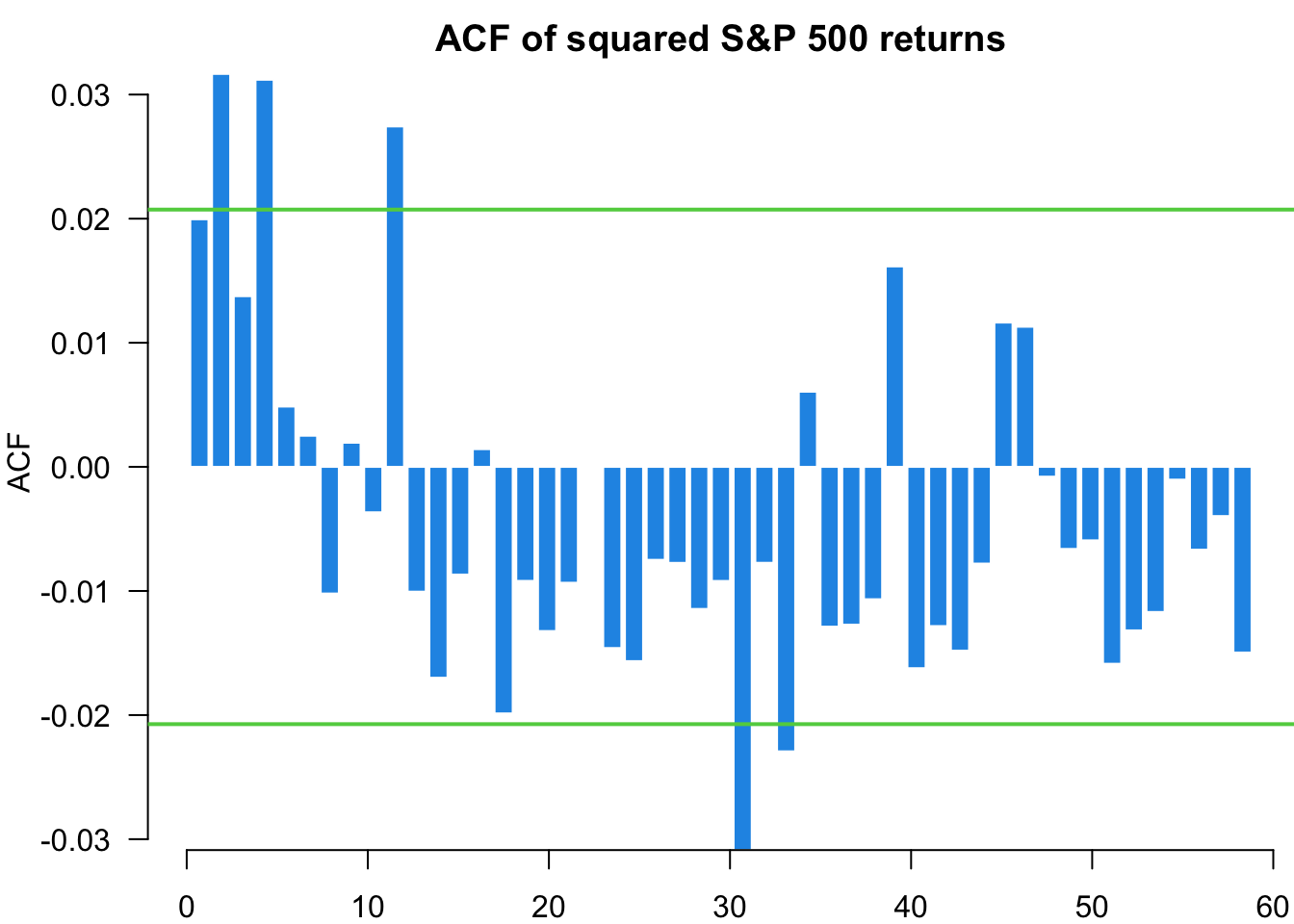
x=qqPlot(residuals, distribution = "norm", envelope = FALSE,main="Normal QQ of S&P 500 returns")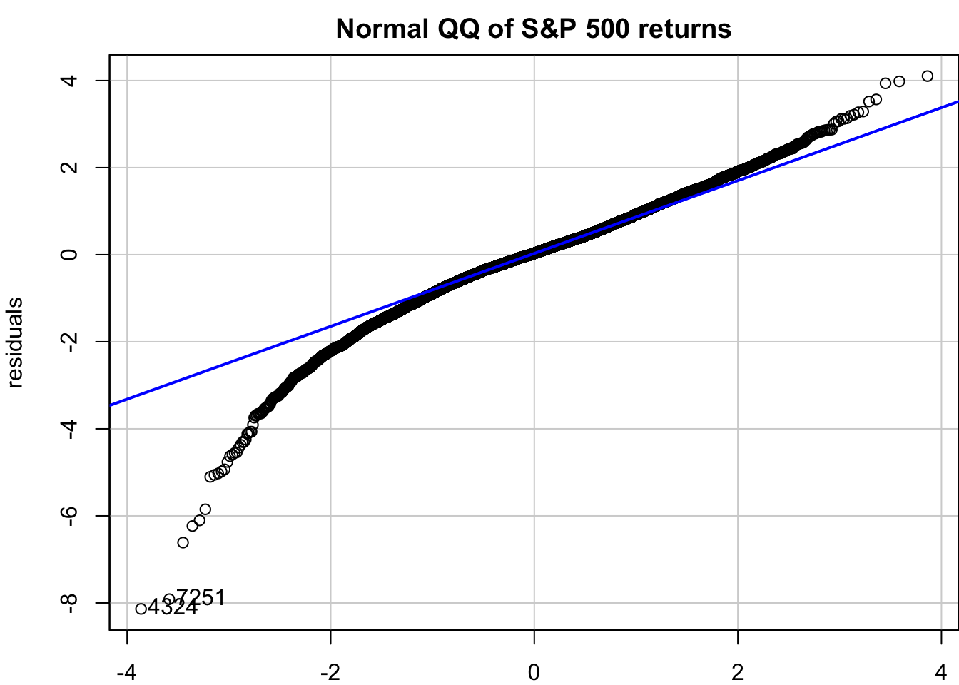
16.7 Monte Carlo analysis of GARCH models
Having estimated and diagnosed our models, we can now explore their properties through simulation. Monte Carlo analysis allows us to generate synthetic data from our estimated models, which is useful for understanding model behaviour, validating estimation procedures, and conducting forecasting exercises.
16.7.1 Using ugarchsim()
16.7.1.1 Gaussian
#| scrolled: true
#| vscode: {languageId: r}
s=ugarchsim(Results$tGARCH11, n.sim = 5000)
par(mar=c(2,3,2,0))
plot(y,type='l',bty='l',las=1,main="S&P 500")
plot(s@simulation$seriesSim,type='l',bty='l',las=1,main="Simulated tGARCH S&P 500")
16.7.1.2 Simulation and estimation
#| vscode: {languageId: r}
N=5
for(n in 1:N){
 s=ugarchsim(Results$GARCH11, n.sim = 5000)
 Results$GARCH11 = ugarchfit(spec = spec.2, data = s@simulation$seriesSim,solver = "hybrid")
 print(Results$GARCH11@fit$matcoef)
}
16.7.2 Manual simulation
While rugarch provides convenient simulation functions, understanding the underlying mechanics through manual implementation is valuable for several reasons. Manual simulation helps verify our understanding of the model structure, allows for custom modifications not available in packaged functions, and provides insight into the iterative nature of volatility processes.
16.7.2.1 GARCH(1,1)
S=1e3
omega=1e-6
alpha=0.15
beta=0.8

N=10000
set.seed(888)
Res=NULL
for(n in 1:N){
 eps=rnorm(S)
 y=rep(NA,S)
 sigma2 = omega/(1-alpha-beta)

 y[1]=eps[1]*sqrt(sigma2)
 for(i in 2:S){
 sigma2= omega+alpha*y[i-1]^2 + beta * sigma2
 y[i]=eps[i]*sqrt(sigma2)
 }


}
par(mar=c(2,3.5,0,0))
plot(y,type='l',bty='l',las=1)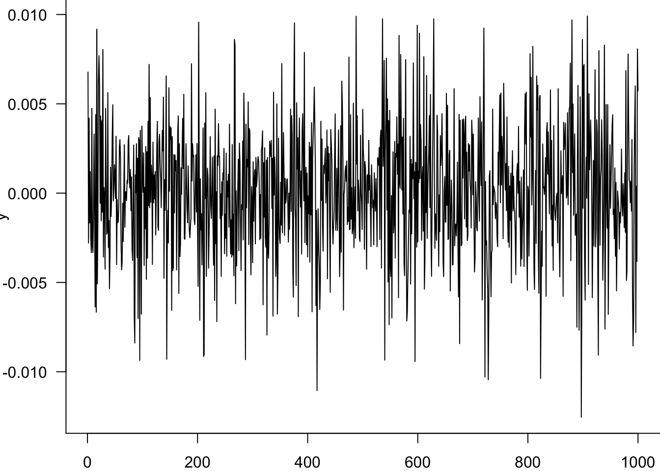
16.7.2.2 tGARCH
df=6
omega=0.000001
alpha=0.15
beta=0.75
N=1
S=1e5
set.seed(888)
for(n in 1:N){
 eps=rt(S,df=df)
 y=rep(NA,S)
 sigma2 = omega/(1-alpha-beta)

 y[1]=eps[1]*sqrt(sigma2)
 for(i in 2:S){
 sigma2 = omega + alpha*y[i-1]^2 + beta * sigma2
 y[i]=eps[i]*sqrt(sigma2)
 }
}
par(mar=c(2,3.5,0,0))
plot(y,type='l',bty='l',las=1)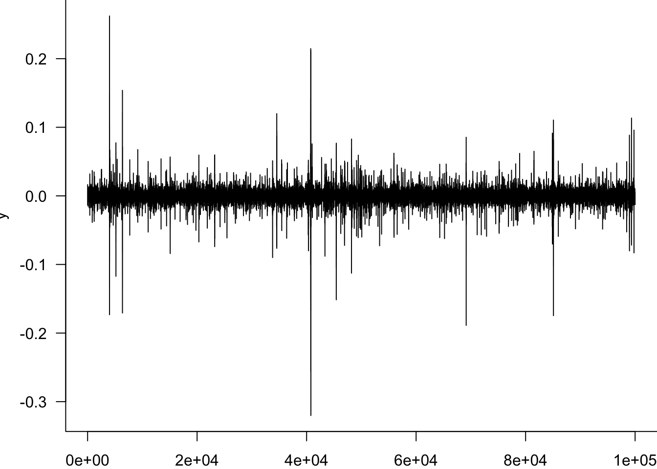
16.8 Exercises
Model comparison: Conduct pairwise likelihood ratio tests for all eight model specifications. Comment on the results and discuss which models provide significant improvements.
Residual diagnostics: For the best-performing model, conduct comprehensive residual analysis including normality tests, autocorrelation tests, and ARCH effects tests.
Forecasting evaluation: Generate one-step-ahead volatility forecasts for the last 100 observations and compare forecast accuracy across different model specifications.
Parameter stability: Investigate parameter stability by estimating your preferred model on rolling windows of 1000 observations. Plot the evolution of key parameters over time.
# Answer
# df.summary refers to the data frame generated in the summary section
library(combinat)
cb=combn(1:8, 2)

rst=c()
for (i in 1:ncol(cb)){
 idx=cb[,i]
 lr.tmp=2*abs(df.summary[1,idx[1]]-df.summary[1,idx[2]])
 pval.tmp=1-pchisq(lr.tmp, df=1)
 rst.tmp=c(lr.tmp, pval.tmp)
 rst=rbind(rst, rst.tmp)
}
colnames(rst)=c("LR Stat", "p-value")
rownames(rst)=1:nrow(rst)
rst
which(rst[,2]>0.05)

# We reject the null hypothesis that the two models are the same for all pairs.