library(reshape2)
library(zoo)
library(rugarch)
source("common/functions.r",chdir=TRUE)20 Implementing risk forecasts
Below, we address the implementation of risk forecast models as discussed in Chapters four and five of Financial Risk Forecasting. This builds directly on the volatility models covered in Chapter 16 and connects to the backtesting framework discussed in Chapter 22.
These risk forecasts provide inputs for more advanced applications including backtesting model performance, portfolio risk aggregation, and regulatory capital calculations covered in subsequent chapters.
The methods implemented here represent common approaches used in practice, from historical simulation to GARCH-based models that capture the stylised facts of financial returns.
Along the way, we will make some functions and add them to functions.r.
20.1 Risk measures: VaR and Expected Shortfall
Value-at-Risk (VaR) and Expected Shortfall (ES) are fundamental risk measures used throughout the financial industry:
VaR answers the question: “What is the maximum loss we expect with probability \(p\) over the next day?” For example, a 5% daily VaR of £100,000 means there is a 5% chance of losing more than £100,000 tomorrow.
ES, also known as Conditional VaR, goes further by asking: “Given that we exceed the VaR threshold, what is the average loss?” ES provides information about tail risk beyond the VaR cutoff.
These measures are commonly used for:
- Regulatory capital requirements (Basel framework);
- Internal risk limits and position sizing;
- Portfolio optimisation and risk budgeting;
- Stress testing and scenario analysis.
The challenge lies in forecasting the distribution of future returns to calculate these measures accurately.
20.2 Data and libraries
data = ProcessRawData()
sp500 = data$sp500
20.3 Specification
When backtesting, we have a number of parameters we have to keep track of, such as probability, portfolio value, sample size, testing window size and estimation window size. In order to minimise the chance of mistakes and make the coding as fast as possible, we use the techniques discussed in Section Section 15.6 and keep track of them in a list that we call par for parameters.
The parameter structure we establish here will be used throughout the risk management chapters, including backtesting (Chapter 22) and portfolio risk analysis. This consistent framework ensures reproducible results across different risk applications.
par         = list()
par$p       = 0.05        # probability level (0.05 = 5% VaR)
par$value   = 1000        # portfolio value in currency units
par$WE      = 2000        # estimation window size (number of observations)
par$T       = length(sp500$y)  # total sample size
par$WT      = par$T-par$WE     # testing window size (T - WE)
par$lambda  = 0.94        # decay parameter for EWMA (0.94 is industry standard)

cat("The backtesting parameters are:",
  "\n\tp =     ",par$p,
  "\n\tvalue = ",par$value,
  "\n\tpar$WE =",par$WE,
  "\n\tT =     ",par$T,
  "\n\tWT =    ",par$WT,
  "\n\tlambda =",par$lambda,
  "\n"
)
The backtesting parameters are:
p = 0.05
value = 1000
par$WE = 2000
T = 8938
WT = 6938
lambda = 0.94 print(par)$p
[1] 0.05
$value
[1] 1000
$WE
[1] 2000
$T
[1] 8938
$WT
[1] 6938
$lambda
[1] 0.9420.4 Functions
While we could program the functionality for backtesting without functions, because we may want to repeat the calculations multiple times and with different parameters, it is much better to use functions. This also allows to reuse them in the Backtesting chapter, Chapter 22.
We label these functions as Risk.* where * refers to any of the methods we are using, like HS or EWMA. We also put these functions into functions.r so we can use them later.
Each function takes three arguments: the returns y, the parameter list par and Print. The Print parameter determines whether the function prints out diagnostic information including the forecast volatility and the calculated VaR and ES values. When set to TRUE, this provides useful feedback for debugging and model validation.
20.5 Historical simulation — Risk.HS
Historical simulation is a method that assumes that history repeats itself. It uses the empirical distribution of the returns to find the \(p\)-th quantile. It assumes that the distribution of past returns represents the future distribution.
par(mar=c(2,3,1,0),bty='l')
plot(sp500$y,type='l',las=1,ylab="Returns",xlab="Time",main="S&P 500 Daily Returns")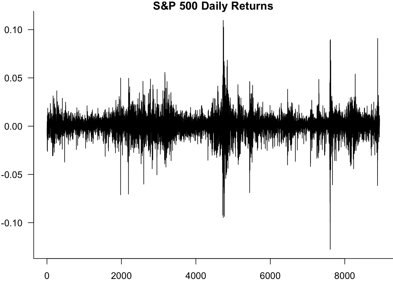
We sort the values using sort():
ys = sort(sp500$y)
par(mfrow=c(1,2))
plot(ys,
    type = "l",
    main="All Sorted Values",
    las=1,
    bty='l'
)
plot(head(ys,50),
    main="The Lowest 50 Sorted Values",
    las=1,
    bty='l'
)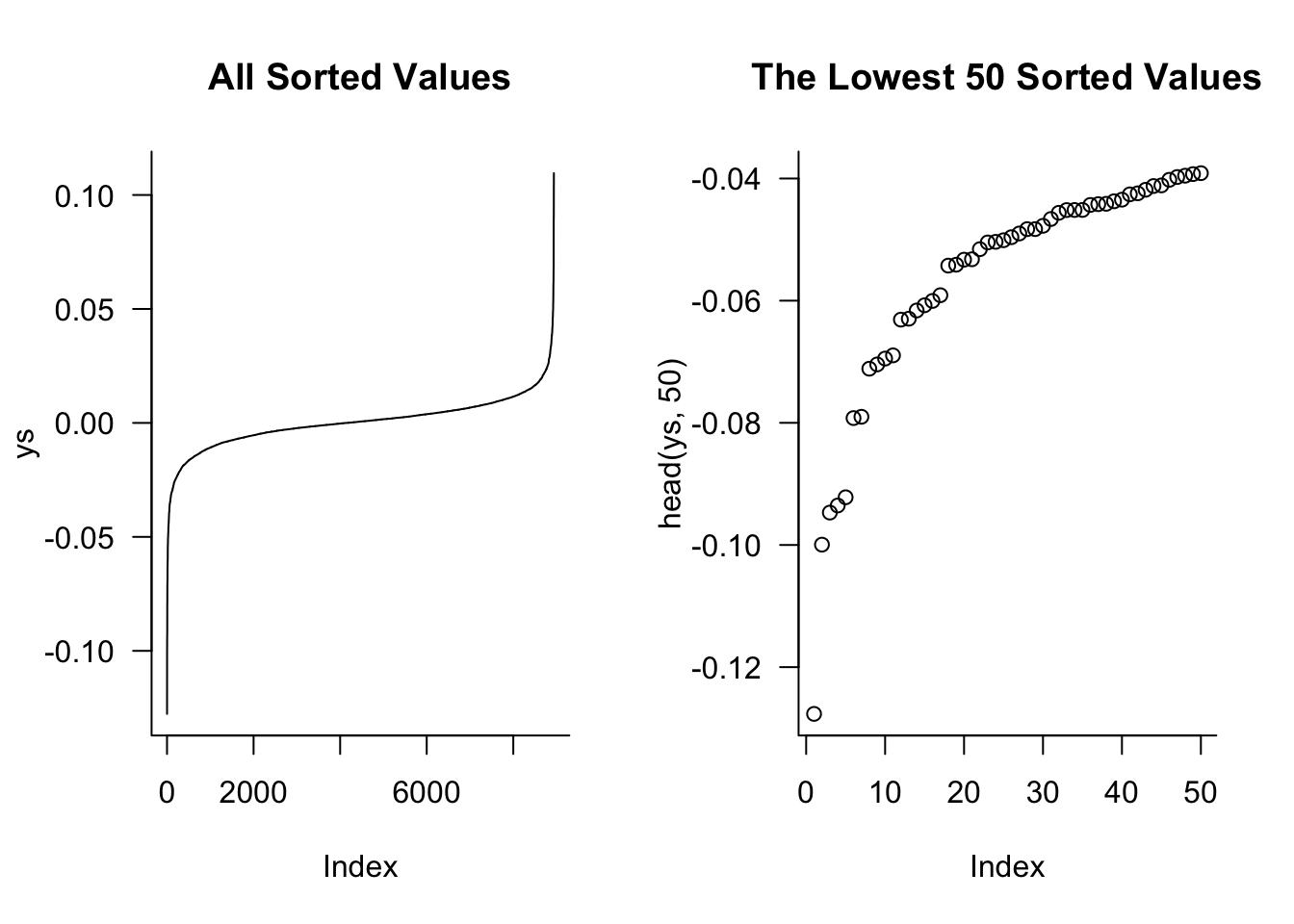
plot(head(ys,60),main="The Lowest 60 Sorted Values",las=1,bty='l')
segments(par$WE*0.01,-1,par$WE*0.01,ys[par$WE*0.01])
segments(par$WE*0.01,ys[par$WE*0.01],0,ys[par$WE*0.01])
segments(par$WE*0.05,-1,par$WE*0.05,ys[par$WE*0.05])
segments(par$WE*0.05,ys[par$WE*0.05],0,ys[par$WE*0.05])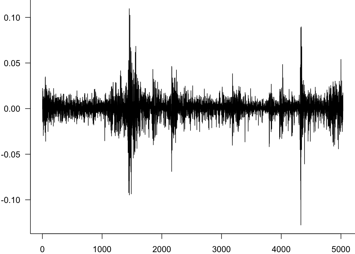
20.5.1 Risk.HS
The function of implementing HS, Risk.HS, is quite straightforward. It takes a vector of returns and the parameter list, along with an optional argument, Print, and returns a list with both the ES and VaR, along with the parameter list.
The Risk.HS function implements historical simulation by sorting the most recent returns and finding the empirical quantile.
Risk.HS=function(y,par,Print=FALSE){
    ys=sort(tail(y,par$WE))
    VaR = -ys[par$p*par$WE] * par$value
    ES = - mean(ys[1:(par$p*par$WE)]) * par$value
    if(Print) cat("The HS ",par$p*100,"% VaR is $",round(VaR,1),", while the ES is $",round(ES,1),"\n",sep="")

    return(list(VaR=VaR,ES=ES,method="HS",par=par))
}
20.6 EWMA — Risk.EWMA
While historical simulation is simple and makes no distributional assumptions, it has limitations. It gives equal weight to all observations in the estimation window and tends to be slow to adapt when market conditions change. The EWMA approach addresses this by giving more weight to recent observations, allowing for faster adaptation to changing volatility.
The Risk.EWMA function uses exponentially weighted moving averages to forecast volatility, giving more weight to recent observations. It assumes returns follow a normal distribution with time-varying volatility.
20.6.1 Normal distribution functions
Since EWMA and GARCH methods assume normally distributed returns, we need functions to calculate VaR and ES from the normal distribution:
NormalVaR=function(p,sd=1) return(-qnorm(p,sd=sd))
NormalES=function(p,sd=1) return(sd*dnorm(qnorm(p))/(p))Risk.EWMA=function(y,par,Print=FALSE){
y = tail(y,par$WE)
sigma2 = var(y)
for (i in 2:length(y)){
sigma2 = par$lambda*sigma2+(1-par$lambda)*y[i-1]^2
}
sigma = sqrt(sigma2)
VaR = NormalVaR(p=par$p,sd=sigma)* par$value
ES = NormalES(p=par$p,sd=sigma)*par$value
if(Print){
cat("The EWMA forecast volatility is",round(sigma,4),"\n")
cat("The EWMA ",par$p*100,"% VaR is $",round(VaR,1),", while the ES is $",round(ES,1),"\n",sep="")
}
return(list(VaR=VaR,ES=ES,method="EWMA",sigma=sigma))
}EWMA improves on historical simulation by weighting recent observations more heavily, but it still assumes a simple exponential decay pattern. GARCH models provide a more sophisticated approach by explicitly modelling how volatility evolves over time, capturing the volatility clustering patterns commonly observed in financial markets.
20.7 Gaussian GARCH
The GARCH approach models volatility clustering by estimating how current volatility depends on past volatility and past squared returns. For details on GARCH estimation, see Chapter 16.
The Risk.GARCH function estimates a GARCH(1,1) model to capture volatility clustering in returns. It uses maximum likelihood estimation and assumes normally distributed innovations.
Risk.GARCH=function(y,par,Print=FALSE){
    ys = tail(y,par$WE)
    y = y-mean(y)
    scale = sd(y)
    y = y/scale
    spec = ugarchspec(
        variance.model = list(
            garchOrder= c(1,1)),
        mean.model= list(
            armaOrder = c(0,0),
            include.mean=FALSE)
    )
    res = ugarchfit(spec = spec, data = y, solver = "hybrid")
    omega = coef(res)['omega']
    alpha = coef(res)['alpha1']
    beta = coef(res)['beta1']
    res@fit$coef[1] = res@fit$coef[1]*scale^2
    sigma = sqrt(omega + alpha*tail(y,1)^2 + beta*tail(res@fit$var,1))* scale
    names(sigma) = NULL
    VaR = NormalVaR(p=par$p,sd=sigma)* par$value
    ES = NormalES(p=par$p,sd=sigma)*par$value

    if(Print){
        cat("The GARCH forecast volatility is",round(sigma,4),"\n")
        cat("The GARCH ",par$p*100,"% VaR is $",round(VaR,1),", while the ES is $",round(ES,1),"\n",sep="")
    }
    return(list(VaR=VaR,ES=ES,method="GARCH",parameters=coef(res),sigma=sigma))
}
While GARCH models capture volatility clustering effectively, they assume normally distributed innovations. This means returns are conditionally normal (given the volatility at time t) but unconditionally exhibit fat tails due to the time-varying volatility. The t-GARCH model goes further by allowing the innovations themselves to follow a Student-t distribution, providing even heavier tails.
20.8 t-GARCH
The Risk.tGARCH function extends the GARCH model by using a Student-t distribution for the innovations instead of normal distribution. This can better captures the heavy tails commonly observed in financial returns.
20.8.1 Student-t distribution functions
An important issue here is whether the Student-t distribution is standardised to have unit variance. Many GARCH libraries standardise the distribution so that variance equals 1, which requires scaling by \(\sqrt{\frac{\text{df}}{\text{df}-2}}\) where \(\text{df}\) is the degrees of freedom parameter.
tVaR=function(p,df,sd=1,Standardized=TRUE){
 Scale=1
 if(Standardized) Scale=sqrt(df/(df-2))
 return(-sd*qt(p=p,df=df)/Scale)
}
tES=function(p,df,sd=1,Standardized=TRUE) {
 Scale=1
 if(Standardized) Scale=sqrt(df/(df-2))
 ES=(sd*dt(qt(p=p,df=df),df=df)*
    ((df+(qt(p=p,df=df))^2)/
    (df-1))/p)/Scale
 return(ES)
}Risk.tGARCH=function(y,par,Print=FALSE){
ys = tail(y,par$WE)
y = y-mean(y)
scale = sd(y)
y = y/scale
spec = ugarchspec(
variance.model = list(
garchOrder= c(1,1)),
mean.model= list(
armaOrder = c(0,0),
include.mean=FALSE),
distribution.model = "std"
)
res = ugarchfit(spec = spec, data = y, solver = "hybrid")
omega = coef(res)[1]
alpha = coef(res)[2]
beta = coef(res)[3]
nu = coef(res)[4]
sigma = sqrt(omega + alpha*tail(y,1)^2 + beta*tail(res@fit$var,1))* scale
res@fit$coef[1] = res@fit$coef[1]*scale^2
names(sigma) = NULL
VaR = tVaR(p=par$p,sd=sigma,df=nu,Standardized=TRUE)* par$value
ES = tES(p=par$p,sd=sigma,df=nu,Standardized=TRUE)* par$value
if(Print){
cat("The tGARCH forecast volatility is",round(sigma,4),"\n")
cat("The tGARCH ",par$p*100,"% VaR is $",round(VaR,1),", while the ES is $",round(ES,1),"\n",sep="")
}
return(list(VaR=VaR,ES=ES,method="tGARCH",parameters=coef(res),sigma=sigma))
}20.9 Application
We now apply all four risk forecasting methods to the S&P 500 data and compare their VaR and ES estimates.
res = list()
res$HS = Risk.HS(y=sp500$y,par=par,Print=TRUE)
The HS 5% VaR is $18.3, while the ES is $30.5res$EWMA = Risk.EWMA(y=sp500$y,par=par,Print=TRUE)The EWMA forecast volatility is 0.01
The EWMA 5% VaR is $16.4, while the ES is $20.6res$GARCH = Risk.GARCH(y=sp500$y,par=par,Print=TRUE)The GARCH forecast volatility is 0.0076
The GARCH 5% VaR is $12.6, while the ES is $15.7res$tGARCH = Risk.tGARCH(y=sp500$y,par=par,Print=TRUE)The tGARCH forecast volatility is 0.0078
The tGARCH 5% VaR is $12.5, while the ES is $17.3for(l in res){
cat(l$method,l$VaR,l$ES,"\n")
}HS 18.31796 30.52792
EWMA 16.42695 20.60006
GARCH 12.55457 15.74393
tGARCH 12.4685 17.28503 for(l in res){
if(l$method==res[[names(res)[1]]]$method){
df = t(data.frame(c(l$method,l$VaR,l$ES)))
}else{
df = rbind(df,c(l$method,l$VaR,l$ES))
}
}
df = as.data.frame(df)
names(df) = c("method","VaR","ES")
rownames(df) = NULL
df$VaR = as.numeric(df$VaR)
df$ES = as.numeric(df$ES)
df| method | VaR | ES |
|---|---|---|
| HS | 18.31796 | 30.52792 |
| EWMA | 16.42695 | 20.60006 |
| GARCH | 12.55457 | 15.74393 |
| tGARCH | 12.46850 | 17.28503 |
The results show notable differences between methods:
- HS typically provides the most conservative estimates, as it relies entirely on past observations without any parametric assumptions about the distribution;
- EWMA estimates tend to be more responsive to recent market conditions due to the exponential weighting scheme, which can result in higher or lower estimates depending on recent volatility patterns;
- GARCH models, both normal and t-distribution, provide estimates based on volatility forecasting that captures clustering effects. The t-GARCH typically gives higher risk estimates than normal GARCH due to the heavier tails of the Student-t distribution.
These differences highlight the importance of method selection based on market conditions, regulatory requirements, and the specific risk management application.
20.10 Method comparison and trade-offs
Each risk forecasting method has distinct advantages and limitations:
HS
- Advantages: Non-parametric, captures actual tail behaviour, simple to implement;
- Limitations: Slow to adapt to regime changes, requires large datasets, equally; weights old and recent observations.
EWMA
- Advantages: Fast adaptation to volatility changes, computationally efficient, industry standard parameters available;
- Limitations: Assumes normal distribution, simple exponential decay may be too restrictive, no long-term mean reversion.
Gaussian GARCH
- Advantages: Captures volatility clustering, theoretical foundation, can incorporate mean reversion;
- Limitations: Assumes normal innovations, requires parameter estimation, may be unstable in small samples.
t-GARCH
- Advantages: Heavy-tailed innovations, better extreme event modelling, maintains volatility clustering,
- Limitations: Additional parameters to estimate, computational complexity, may overestimate risk in calm periods, volatile risk forecasts.
The choice between methods depends on data availability, computational constraints, regulatory requirements, and market conditions.
20.11 Exercises
Create a generic function for obtaining VaR and ES from GARCH models, where the particular model specification, normal, t, skew t, lags, and apARCH, are arguments to a single function.
Combine all risk functions discussed above into a single function,
Risk = function(y,par,Model,Print), that computes ES and VaR based on a set of inputs. This function should support HS, EWMA, GARCH, and tGARCH models and be robust enough to handle improper inputs.